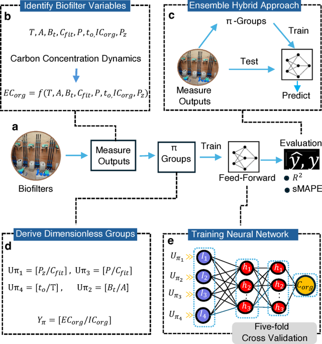
Figure 1a, provides a detailed visualization of the EnviroPiNet framework, showcasing how outputs from the biofilter are measured and processed.
The dataset was generated by collecting data from drinking water biofilters, capturing variables such as \(T\), the temperature of the water at the sample location; \(P_z\), the pore size of the sample, representing the characteristic diameter of the voids or pores within the biofilter material; \(A\), the age of the filter measured as the time from the start of the experiment; \(IC_{\text {org}}\), the influent carbon concentration of the sample; \(EC_{\text {org}}\), the effluent carbon concentration of the sample; \(B_t\), the empty bed contact time, which is estimated at the start of the experiment and assumed to be constant for each filter; \(P\), the average diameter of the granular activated carbon (GAC) particles; \(C_{\text {fit}}\), the diameter of the filter bed, which is a constant for each filter; \(t_o\), the ambient air temperature, which is assumed to be constant for all locations in the bed at each time point. The units and dimensions of these parameters are shown in Table S1 (available in the Supplementary Methods). Each instance is a unique realisation of this vector of variables. These variables were systematically recorded over time to ensure robust and comprehensive data representation.
To evaluate the models’ predictions of organic carbon concentrations in the effluent, three time series datasets were combined for training. The time series are sparse; therefore, we combined all three datasets for training and set aside (20%) of the combined data, derived from the third dataset, for evaluation. The primary training dataset originates from Quinn , encompassing 175 observations over 162 days, with measurements of chemical composition, microbiology, and temperature taken weekly for the first 12 weeks and biweekly thereafter. Additionally, data from15 contributed 26 instances of the same observed variables. This study explored the impact of biofilter design and operational conditions on bacterial community composition and abundance in pilot-scale biofilters. Different filter media (granular activated carbon-sand versus anthracite-sand) and backwashing strategies were analyzed over 18 months of operation. The experimental setup included parallel operation of six replicate columns, ensuring robust assessments of the effects of media type and operational conditions. The dataset from16 added 116 samples, of which 54 observations were included in the training set. This study investigated five laboratory-scale biofilters with varying operational temperatures (\(10^{\circ }\)C and \(20^{\circ }\)C) over 48 weeks. The biofilters were packed with Norit® GAC 1240 and operated with an empty bed contact time of 3 h. Measurements of influent and effluent water quality parameters were taken weekly during the first 12 weeks and every six weeks thereafter. For testing, 62 observations from16 were reserved, forming a completely independent evaluation dataset. To ensure consistency, the dimensional data were transformed into dimensionless data using Equation S8. Details of the testing dataset are outlined in Details of the testing dataset are outlined in Table S2 (available in the Supplementary Methods).
In Fig. 1b, we highlight the identification and selection of key biofilter variables. The models relied on measured variables common to all studies, necessitating the exclusion of potentially useful information specific to individual studies. These variables were then used to formulate the equation, where the carbon concentration function is expressed as a combination of independent variables. In Fig. 1d, we illustrate the systematic approach of Buckingham Pi theorem to generate dimensionless \(\pi\)-groups from the selected variables. This approach simplifies the dataset while preserving the essential physical relationships between variables. The first part of EnviroPiNet generates \(\pi\)-groups (Equation S8), which are compared with two other methods, PCA (Eq. 2) and Autoencoder (Eq. 3), that reduce features to a smaller set of variables without preserving the physical relationships between them. The reduced variables are then used as inputs to a neural network or linear regression model, which determines the coefficients of the monomial model. Fig. 1c then highlights the process of feeding the \(\pi\)-groups into a neural network. After standardizations the \(\pi\)-groups, they are used as inputs to the neural network to predict carbon concentration, a crucial step for developing an accurate and generalizable predictive model. Finally, Fig. 1e, depicts the architecture of the feedforward neural network employed in EnviroPiNet. This architecture was designed to capture nonlinear relationships in the data, enhancing the model’s predictive performance for carbon concentration dynamics. The neural network training utilized 5-fold cross-validation, ensuring that after each epoch, a measure of goodness of fit was calculated for a randomly allocated 80% portion of the data used for training. Additionally, a second measure was computed using the remaining 20% of the data reserved for validation. These measures were plotted over the epochs to generate the loss plots. Supplementary Fig.S1 presents the loss plots for EnviroPiNet, using two metrics: Mean Squared Error (MSE) Supplementary Fig.S1.a and Mean Absolute Error (MAE) Supplementary Fig.S1.b. These curves illustrate the convergence of both training and validation measures, suggesting that the model effectively learns from the training data and generalizes well to unseen validation data. For the PCA-NN, KPCA-NN, and Autoencoder-NN models, the loss curves in supplementary Fig.S1.c and Fig.S1.e demonstrate that the models effectively learn from the training data and generalize well to the validation data. The corresponding Mean Absolute Error (MAE) values are presented in supplementary Fig.S1.d and Fig.S1.f, respectively.
However, as seen in Table 1, it does not perform well on unseen test data. This could be because, during training, the model is trained, tuned, or adjusted based on the validation performance. Since PCA and autoencoders focus on capturing the most significant variance in the data, they may ignore less prominent but still important features that are crucial for predicting the target variables. The proportion of variance captured by the first few principal components is shown in Fig.S2. Therefore, the validation data may exhibit the same general patterns as the training data, which allows the model to perform well during training. However, when we apply the model to completely unseen test data, the test data may contain patterns or variations that were not captured well by the dimensionality reduction techniques, leading to poor performance on the unseen data.The architecture and dimensionality reduction behavior of the autoencoder are illustrated in Fig.S3, which shows how eight input variables are compressed into four latent variables used for prediction. Typically, K-fold cross validations are not applied for regression analyses, rather a single goodness of fit is reported for the model using training data.
The trained models were applied to the unseen test dataset from study16. Thus, the reduced variates are calculated from the raw data and then the trained neural neworks, with trained node weights unchanged, and the monomial models, with the trained exponents, are applied. Again, we can calculate the various performance metrics can be calculated. The R2 and sMAPE metrics are compared for the models appled to the trainind and test datasets in Tables 1 and 2 respectively.
For Autoencoder reduced set of variates the relationship to the original variables can be nonlinear and is difficult to interpret in any biological or physical way. The reduced set of PCAs are orthogonal linear combinations of the orginal expanatory variables and thus are slightly easier to interpret in terms of the biology and physics. Buckingham Pi variates are, in effect, selected to encapsulate the science of the system. Thus, especially when used in an analytic functional form, their influence on the independent variable can be interpreted. The linear regression fitted exponents for the BP-LR are reported:
$$\begin{aligned} \frac{\textrm{EC}_{\textrm{org}}}{\textrm{IC}_{\textrm{org}}} = \text {intercept} \left( \frac{P_z}{C_{\textrm{fit}}} \right) ^{-0.06} \left( \frac{B_t}{A} \right) ^{-0.30} \left( \frac{P}{C_{\textrm{fit}}} \right) ^{0.53} \left( \frac{t_0}{T} \right) ^{-0.09} \end{aligned}$$
(1)
Where the intercept is the estimated constant, given by \(\exp (-0.07) = 0.93\), and each term in the equation represents the effect of different variables on the organic carbon concentration in the treated water. The model suggests that changes in \(\frac{P}{C_{\textrm{fit}}}\) have a large effect on the proportion of carbon removed in the filter. Thus, the smaller radius of GAC particles and the greater the radius of the filter (a surrogate for the amount of GAC) result in more carbon removed. Given that this variable relates to the surface area of activated carbon, this makes sense. The ratio \(\frac{B_t}{A}\) is raised to the power \(-0.3\), meaning that as \(A\) increases, the proportion of carbon removed decreases, and thus, the older the filter, the poorer the treatment. Changes in \(P_z\) and temperature have a smaller effect on carbon removal.
In addition to the results presented, Fig. 2a, b provide visual representations of the linear regression plots for the test dataset, comparing the EnviroPiNet and BP-LR models. Figure 2a showcases the Pearson correlation coefficient (r-value) of \(0.97\) with \(p < 0.05\) for EnviroPiNet, along with an R-squared value of 0.9. Figure 2b demonstrates an r-value of 0.86 with \(p < 0.05\) for BP-LR, along with an R-squared value of 0.34. These figures emphasize the distinct characteristics and performance metrics of each model when evaluated on the test data.
In this study, we aimed to predict the carbon concentration \(EC_{\text {org}}\),in drinking water biofilter effluent. The Environmental Buckingham Pi Neural Network (EnviroPiNet) demonstrated superior performance for predicting \(EC_{\text {org}}\),achieving an \(\text {R}^{2}\) value of 0.9, as shown in Table 1, and a sMAPE value of 6, as presented in Table 2. The model also yielded a Pearson correlation coefficient r -value) of 0.97 with a p-value less than 0.05, as depicted in Fig. 2a. The corresponding learning curve is illustrated in Fig. 1a. In comparison, linear regression (BP-LR) was applied, resulting in a Pearson correlation coefficient r-value of 0.86 with a p-value less than 0.05, as shown in Fig.2b, an \(\text {R}^{2}\) value of 0.34, as presented in Table 1, and a sMAPE value of 10, as shown in Table 2, for the prediction of \(EC_{\text {org}}\). Additionally, ensemble methods such as Gradient Forest Regression (BP-GFR), Random Forest Regression (BP-RFR), and Support Vector Regression (BP-SVR) were evaluated, each yielding a Pearson r r-value of approximately 0.7.
The results show that the EnviroPiNet model’s \(\text {R}^{2}\) value outperformed the linear regression model. This suggests that the EnviroPiNet benefited from the Buckingham Pi theorem, enabling it to leverage the advantages of learning from a low-diversity dataset while using the neural network to capture nonlinear and complex relationships. Consequently, it outperformed linear regression in this specific application, as shown in Fig. 2c. An ablation study was conducted to assess the impact of physics-guided Buckingham Pi features on model performance. The EnviroPiNet neural network was trained on both the Buckingham Pi-transformed inputs and the original raw input variables. Performance metrics on the test set are summarized in Table S5. The model trained on Buckingham Pi groups achieved a higher \(\text {R}^{2}\) and lower sMAPE compared to the model trained on raw variables, demonstrating the added value of physics-based feature engineering.To further examine the contribution of individual features, SHAP analysis was performed on the training data using a Ridge regression model with Buckingham Pi features. The SHAP summary and bar plots (Figs. S4 and S5) indicate that features \(U\pi _2\) and \(U\pi _4\) consistently contribute significant positive and negative impacts on predictions, respectively. Waterfall plots for individual observations (Fig.S6) reveal variation in feature contributions across samples, with \(U\pi _2\) ranging from –0.19 to +0.38 and \(U\pi _4\) from approximately –0.11 to +0.18. The alignment of SHAP values with the model’s predicted and expected outputs supports the physical relevance of these Buckingham Pi groups in predicting \(\textrm{EC}_{\textrm{org}}\). Details about the SHAP analysis setup are provided in the Supplementary Methods.