Researchers presented many studies that contribute to predicting software cost estimates, but their results were not accurate or satisfactory enough, so the study sought to build a model based on artificial intelligence techniques in its mechanisms. The study sought to use machine learning and deep learning techniques by using a convolutional neural network to predict software cost estimates and improve network performance through particle swarms for optimization, which in turn contributes to parameter optimization. The proposed study includes an organized and interconnected series of procedural steps that aim to enhance reliable predictive results, as shown in Fig. 2.

The process entails collecting permanent datasets through a systematic data collection phase. Next, it involves comprehensive data analysis, including descriptive statistics, preprocessing techniques, exploratory data visualization, and identification of distinct training and test sets, culminating in data normalization through scaling procedures. The subsequent phase involves the custom development of a CNN architecture specifically designed for cost estimation purposes. After the architecture is designed, the PSO is set to optimize the hyperparameters, including iterative parameter generation, fitness function formulation, algorithmic implementation, and optimal hyperparameter extraction, thus enhancing the CNN performance. After hyperparameter optimization, rigorous training of the model is performed using the custom training dataset. When training is finished, the normalization process is reversed to restore the data to its original state. The final evaluation of model performance comes from a comprehensive evaluation that uses six distinct evaluation metrics, including mean absolute error (MAE)29, mean square error (MSE)30, root mean square error (RMSE)31, mean magnitude of relative error (MMRE)32, median magnitude relative error (MDMRE)33, and prediction accuracy (PRED)34. This rigorous methodological framework represents a scientific endeavor aimed at enhancing the accuracy and reliability of software cost estimation models.
Implementing the proposed methodology for software cost estimation is intertwined with several challenges, each of which necessitates comprehensive examination to ensure its effectiveness and robustness in practical contexts. These challenges span diverse dimensions, each of which requires careful attention and strategic mitigation strategies to support the credibility and applicability of the methodology. The challenge of data availability and quality is that procuring comprehensive and unbiased datasets is extremely challenging, given the inherent variability and potential biases in data sources. Data quality issues, such as incompleteness or skewed distributions, greatly impact the accuracy and generalizability of predictive models and the challenge has been addressed by using data scaling to keep data within a single context and have close, eligible values during processing.
The second challenge is computational complexity, as combining a convolutional neural network (CNN) architecture with particle swarm optimization (PSO) introduces significant computational requirements, especially during hyperparameter optimization. It requires effective management of computational complexity. The challenge was met by customizing optimization strategies to ensure practical feasibility and scalability. The problem of sensitivity of hyperparameter tuning also arises, in which hyperparameter tuning using PSO is vulnerable to changes in initial conditions, which emphasizes the importance of rigorous experimentation and validation procedures. The use of powerful optimization algorithms and validation techniques is essential to achieve stable and optimal model performance amid hyperparameter sensitivity. It also shows the challenge of overfitting and generalization in which achieving a careful balance between model complexity and generalization performance is crucial to mitigate overfitting. Techniques such as regularization and cross-validation serve as indispensable tools to ensure that developed models generalize well to unseen data while overfitting challenges. Comprehensively addressing these challenges is crucial to enhancing the credibility and practical utility of the proposed methodology in software cost estimation research endeavors.
Datasets
It was based on 13 benchmark datasets that are publicly available and easily accessible via the Promise25 and GitHub26 repositories. These datasets are specifically used to estimate the effort and cost of software and have a close relationship with the literature, as all previous studies depend on them, so they are suitable for evaluating the proposed model. Their sizes range from small to medium to large to suit all types of projects that the model can predict. Its features range from 6 as the minimum number of features used to 24 features as the largest number of features to train the proposed model. This adds great diversity to prove the efficiency of the proposed model, as shown in Table 2 which is not limited to that only, but provides several columns representing the name of the datasets used, the source of the repository from which the datasets were collected, the number of projects for each project, in addition to the number of features, the number of missing values, and the effort output of each dataset, whether monthly or hourly, through which the cost is estimated. Software. It is clear from seeing the statistics that there is a difference in the size of the data, as Albrecht, Kemmerer, and Miyazaki are considered small datasets, while China, Kokomo, Maxwell, and Kokomo are medium and large datasets.
Data analysis
Data description
Firstly, datasets are uploaded to Google Drive as data files and then read and added through Google Colab50. This study uses the read CSV() function to read those files. The info() function is also used to find out all the information about the data used, such as the number of rows and columns and whether there are null values. To understand the data statistically and distribute it, this study uses the describe() function to standardize the values and ensure that they are all numerical. At the end of the analysis process, a copy of the datasets is made to be used in that process to preserve the basic data. To complete the process, use the copy () function.
Data preprocessing
After reading the data, the preprocessing phase begins to eliminate errors, inconsistencies, missing values, as well as outliers51. First, all values are converted to numerical, as the dev_mode attribute is converted from object to numerical. The data is also converted sequentially to be linked, with the time attribute set as an index for the data sequence. In addition, the absence of null values is also checked by the isnull().sum() function.
Data visualization
Data is represented to determine the extent of communication and interrelation between that data. Each attribute is represented by two horizontal and vertical axes, representing the extent of correlation between these variables52. This is reported by the corr() function. To produce a set of values in a certain range. If the result between the correlations of the two variables is equal to one, this means that the relationship between them is very strong. If it is equal to zero, it means that there is no relationship between them. However, if the result is a negative value, the relationship between them is inverse.
Time series forecasting
Time series forecasting is a method of predicting future values based on previous observations of the variable and includes analysis of historical data to identify patterns and trends that can then be used to build a forecasting model. It includes several common methods, including neural networks used in the proposed model. It is widely used in finance, economics, weather forecasting, and many other fields. It is very important to evaluate the performance of the chosen method and take into account factors such as data quality and seasonality when performing time series forecasting53.
Time series forecasting begins with the preprocessing phase of critical data, which identifies the time dimension as a pivotal factor in cost analysis. By converting the time column to date-time format and then indexing the data accordingly, the chronological order of the program cost data is preserved, laying the foundation for rigorous time series analysis. Through techniques ranging from traditional statistical methods to advanced machine learning algorithms, historical cost trends are leveraged to forecast future spending patterns. This predictability empowers project stakeholders with proactive decision-making tools, enabling them to overcome the uncertainties inherent in software development projects. Time series forecasting is emerging as an indispensable tool in the software cost estimation arsenal, providing a data-driven approach to enhance project planning and execution.
Data splitting
This process is also called data partitioning. The data is divided into distinct groups for specific purposes. In this study, it is divided by 20–80% to be the largest percentage for the training process, where the model is trained on that data. The remaining 20% of the data is used in the testing process to measure the accuracy of the proposed model.
Data scaling
It is also called the process of data normalization or standardization which is used to convert the numeric features of a dataset to a common scale. This method is used so that the algorithm can handle all values and not ignore them, especially if they are high values.
Build CNN model
Convolutional neural networks (CNNs) represent a massive class of deep learning models precisely designed to address the complex challenges inherent in analyzing images, video, and digital data such as time series or tables. These networks are characterized by a multi-layer architecture, comprising complex arrangements of convolutional layers, pooling layers, and densely connected layers, which are collectively designed to facilitate the extraction and interpretation of complex patterns. CNNs have emerged as a cornerstone, capturing the attention of researchers and achieving groundbreaking advances in data processing20. The central layers of the CNN framework, as shown in Fig. 3, lie in the convolutional layers, which serve as the underlying mechanism for extracting features from the raw input data. These layers work similarly to a complex set of digital filters, carefully examining the input and distinguishing the signals. Through a process of mathematical convolution, each convolutional layer produces a feature map, encapsulating salient aspects of the input content. Moreover, the subsequent integration of pooling layers within the CNN architecture facilitates hierarchical organization and densification of extracted features, thus enhancing computational efficiency and enabling robust representation learning. At their core, CNNs embody a cutting-edge blend of mathematical abstraction and computational prowess, revolutionizing the AI-powered data analysis landscape54.

Mathematically, the convolution operation within a CNN is denoted as in Eq. (1):
$$\left( {I*K} \right)\left( {p, q} \right) = \Sigma \Sigma I\left( {m, n} \right)K\left( {p – m, q – n} \right)$$
(1)
where I represents the input, K denotes the kernel, and * signifies the 2D convolution operation, with (p, q) denoting the position within the resulting feature map.
In the convolutional layer, the resultant feature map C is computed as in Eq. (2):
$$C\left( {p,q} \right) = f\left( {\Sigma \Sigma K\left( {m,n} \right)I\left( {p – m,q – n} \right) + b} \right)$$
(2)
where f represents the activation function, such as rectified linear unit (ReLU), and b signifies the bias term.
Pooling, a subsequent operation within CNNs, is described in Eq. (3):
$$P\left( {p, q} \right) = \max \left( {I\left( {m, n} \right)} \right) for m \in \left[ {r, r + s} \right), n \in \left[ {t, t + s} \right)$$
(3)
where P denotes the output of the pooling operation, while r and t represent the coordinates of the pooling window’s top-left corner, with s indicating the window size.
The fully connected layer, a pivotal component of CNNs, is articulated in Eq. (4):
$$Y = f\left( {WX + b} \right)$$
(4)
where Y signifies the output, W represents the weight matrix, X denotes the input vector, and b indicates the bias term.
When composing the neural network architecture, specific choices were made regarding the size of the network and the choice of activation functions based on experimental evidence and theoretical considerations. The proposed model is designed as a sequential set of layers within the tensorflow (tf) framework as in Fig. 4. It consists of the following layers55,56,57:
-
Convolutional layer (Conv1D): this layer is generated with 64 filters and a kernel size of three, using a modified linear unit (ReLU) activation function. Previous research indicates that deeper networks with increased filtering capabilities can effectively capture complex patterns within time series data. Convolutional layers are adept at capturing local spatiotemporal patterns inherent in sequential data. The model can effectively extract diverse features while introducing the nonlinearity of the ReLU activation function needed to learn complex relationships within the data. The input format is specified as (n_steps, 1), where n_steps represents the number of time steps in the input data as it is represented by five steps. The input format is designed to suit the sequential nature of the data, ensuring compatibility with convolutional operation while encapsulating each data point as an individual feature.
-
Pooling Layer (MaxPooling1D): a pooling layer with pool size two is applied after the convolutional layer to sample the feature maps. MaxPooling makes it easy to reduce spatial dimensions while preserving prominent features. Using pool size helps achieve computational efficiency and mitigates overfitting by retaining the most useful features.
-
Normalization layer: this layer is responsible for normalizing multi-dimensional feature maps into a one-dimensional matrix, and preparing them for input into subsequent fully connected layers. Flattening allows subsequent fully connected layers to receive feature representations in a flattened format, which simplifies the process of extracting higher-level patterns from the data.
-
Dense layers (fully connected layers): a dense layer containing 32 units and a ReLU activation function is used to transform the features. Fully connected layers capture general patterns within the learned features, enhancing the model’s ability to map features to the target variable. This increases the model’s ability to distinguish complex patterns within the data.
-
Output layer: the final output layer consists of a single module, suitable for regression tasks. A single output unit is well suited because it enables the model to directly predict continuous values, consistent with the goal of regression analysis.
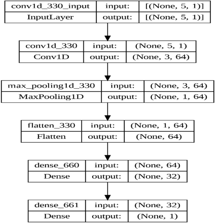
The visualization of the proposed CNN model.
This model architecture embodies a simplified approach to processing one-dimensional sequential data, such as time series, with a combination of convolutional and pooling layers for feature extraction and dimensionality reduction, followed by dense layers to represent higher-level features and regression outputs.
CNN is used in many fields as it is used in the software industry. Cong Pan et al.58 presented models based on it to predict software defects, find errors in programs, and prioritize testing efforts. Jian Li et al.59 also used it to predict software defects, but he improved the model by linking it to the DP model to produce a CNN DP model that shows an improvement in results of 12% compared to previous studies. The model was also used to predict software defects and errors by Wongpheng et al.60, and experimental results showed that CNN was promising for predicting defects with an average accuracy of 70.2%. It has also been used to solve problems in software engineering, such as detecting code smells, which cause an increase in technical cost and negatively affect the software. Lui et al.61 used CNN techniques to detect code smells to improve accuracy and detect different types of smells.
The particle swarm optimization (PSO) algorithm
Particle swarm optimization (PSO) algorithm is a stochastic population-based optimization technique that mimics the social behavior of a flock of birds or schooling fish and is particularly inspired by aggregation or swarming behavior observed in nature21. PSO was introduced by Kennedy and Eberhardt in 199562 and has gained significant attention due to its simplicity and effectiveness in solving various optimization problems. In PSO, a set of candidate solutions, known as particles, iteratively searches the solution space guided by its own experiences and those of its neighbors. Each particle adjusts its position and velocity according to its best-known location and the best-known locations within its neighborhood. The movement of particles toward optimal solutions is governed by two main components: the cognitive component (exploitation), which represents the particle’s tendency to move toward its personal best solution, and the social component (exploration), which represents the particle’s tendency to move toward optimal solutions. The best solution worldwide. Found by her neighbors. This balance between exploration and exploitation enables PSO to efficiently explore the solution space while converging toward promising regions63.
PSO dynamics are governed by various parameters such as swarm size, inertial weight, cognitive and social learning factors, and topology that determine the neighborhood structure. These parameters play critical roles in determining an algorithm’s convergence speed, its exploration–exploitation trade-off, and its robustness in different problem domains. Extensive research has been conducted to study the effect of parameter settings and propose adaptive strategies to adjust these parameters during the optimization process dynamically. In addition, several variants and extensions of PSO have been proposed to enhance its performance, including hybrid approaches that combine PSO with other metaheuristic techniques, constraint-handling mechanisms, and parallel implementations64.
In PSO, each potential solution, known as a particle, adjusts its position and velocity in the search space based on its own experience and the experiences of its neighbors. The position of particle i at iteration t, as in Fig. 4, is represented by \({x}_{i}^{t}\). And its velocity by \({v}_{i}^{t}\). Each particle maintains its best-known position \({p}_{i}^{t}\), and the global best-known position among all particles is denoted as \({p}^{global}\).
The velocity update equation for particle i at iteration t in PSO is given by Eq. (5):
$$v_{i}^{t + 1} = w \cdot v_{i}^{t} + c1 \cdot r1 \cdot \left( {p_{i}^{t} – x_{i}^{t} } \right) + c2 \cdot r2 \cdot \left( {p^{global} – x_{i}^{t} } \right)$$
(5)
where w is the inertia weight controlling the impact of the previous velocity, c1 and c2 are the cognitive and social learning factors, controlling the particle’s tendency to follow its personal best and the global best position, respectively. r1 and r2 are random values drawn from a uniform distribution in the range [0, 1].
The position update equation for particle i at iteration t is then given by Eq. (6):
$$x_{i}^{(t + 1)} = x_{i}^{t} + v_{i}^{(t + 1)}$$
(6)
To update the personal best position (\({p}_{{best}_{i}}\)) of particle i and the global best position (\({\text{g}}_{best}\)), the following Eqs. (7), (8) are employed:
$$p_{{best_{i} }}^{t + 1} = \left\{ {\begin{array}{*{20}c} {p_{{best_{i} }}^{t} } & {if\, f\left( { p_{{best_{i} }}^{t} } \right) \le f\left( {p^{t + 1} } \right)} \\ {x_{i}^{t + 1} } & {if\, f\left( { p_{{best_{i} }}^{t} } \right) > f\left( { x_{i}^{t + 1} } \right)} \\ \end{array} } \right\}$$
(7)
$$g_{b} est^{(t + 1)} = \max \left\{ {f\left( y \right) , f\left( { g_{best}^{t} } \right)} \right\}where\, y \in \left\{ {p_{{best_{0} }}^{t} , p_{{best_{1} }}^{t} , \ldots , p_{{best_{n} }}^{t} } \right\}$$
(8)
Through these equations, particles iteratively explore the solution space, aiming to converge toward optimal solutions while balancing exploration and exploitation as shown in Fig. 5.

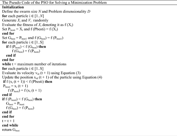
The presented pseudocode defines the operational framework of PSO to solve minimization problems. Its importance is multifaceted. Where you follow a set of steps65:
-
1)
Structured initialization: the algorithm begins with a systematic initialization phase, where basic parameters such as swarm size and problem dimensions are determined. This phase sets the foundational framework for subsequent iterations.
-
2)
Random generation of particle features: the pseudocode provides for the random generation of particle positions and velocities, a crucial step that imparts randomness to the algorithm, allowing exploration of the solution space.
-
3)
Fitness evaluation: the fitness of each particle is evaluated based on its current position, providing a metric to measure its performance within the problem domain. This assessment is pivotal in directing the improvement process towards areas of improved fitness.
-
4)
Dynamic updating of particles and global best positions: through iterative optimization, particles constantly update their personal best positions based on their fitness evaluations. At the same time, the algorithm dynamically adjusts the global best position, reflecting the collective optimization progress of all molecules.
-
5)
Iterative optimization: the essence of the PSO algorithm lies in the iterative optimization process, where particles repeatedly adjust their velocities and positions to efficiently explore the solution space. This iterative optimization facilitates convergence toward optimal solutions over successive iterations.
PSO pseudocode serves as a foundational blueprint for developing effective optimization strategies, as its importance extends to its structured configuration, iterative optimization process, and applicability across diverse problem domains. Through its systematic approach to exploring and exploiting solution spaces, PSO contributes to the development of computational problem-solving methodologies.
The PSO algorithm has been used in similar studies, where Vahid et al.66 used it to estimate development efforts by combining it with Analogy-based estimation to increase the accuracy of estimating software development efforts. However, ABE is unable to produce accurate estimates when the level of importance of project features is not the same or when the relationship between features is difficult to determine. However, the results were promising by combining PSO and ABE and contributed significantly to the estimation.
Among similar studies, Windisch et al.67 presented a method for creating a test that achieves high coverage of structured code. PSO was used to search for relevant test cases. Experiments were conducted on 25 small industrial test objects and 13 more complex artificial test objects taken from different development projects. The algorithm has been shown to outperform most of the code elements to be covered in terms of effectiveness and efficiency.
Combining CNN with PSO
The integration of particle swarm optimization (PSO) algorithm with convolutional neural networks (CNNs), as in Fig. 6, presents a distinctive approach for optimizing hyperparameters in machine learning tasks, particularly in the realm of time series forecasting. The fitness function, which encapsulates the performance evaluation of the CNN model, dynamically adjusts key parameters such as learning rate, number of epochs, optimizer type, and batch size, thereby facilitating the exploration of the hyperparameter space68.

The flowchart of the combination of CNN with PSO.
In this combination, a CNN model is constructed using tensorflow’s Keras API, comprising layers tailored for time-series data analysis. Specifically, the model architecture includes a one-dimensional convolutional layer with 64 filters and ReLU activation, followed by max-pooling and flattening layers to extract relevant features. Subsequently, two dense layers with ReLU activation are added to facilitate learning, culminating in an output layer for regression tasks.
To optimize the model’s performance, PSO is employed to search for the optimal combination of hyperparameters. Through iterative updates guided by the fitness function, PSO navigates the hyperparameter space to identify configurations that minimize the validation loss, thereby enhancing the model’s predictive accuracy and generalization capability69.
Upon completion of the PSO optimization process, the best-performing hyperparameters are retrieved for further analysis and model refinement. These hyperparameters, including the optimal learning rate, number of epochs, optimizer type, and batch size, are crucial determinants of the CNN model’s efficacy in capturing intricate patterns within the time series data.
The fusion of PSO with CNNs offers several advantages in the context of time-series regression tasks. Firstly, it enables automated hyperparameter tuning, reducing the manual effort required for parameter selection and fine-tuning. Secondly, by exploring a diverse range of hyperparameter configurations, PSO enhances the robustness and generalization capability of the CNN model, leading to improved predictive performance on unseen data. Additionally, the iterative nature of PSO allows for efficient exploration of the hyperparameter space, facilitating the identification of optimal configurations within a reasonable computational budget.
The sequential implementation of the provided set is done through the definition of the fitness function, which serves as a corner reservation for evaluating the performance of the CNN. It accepts a set of parameters, including learning rate, epochs, optimizer type, and batch size, as input. The CNN model is created using tensorflow’s Keras API, which is precisely configured using layers specifically designed for analyzing time series data. The model undergoes clustering using the specified optimizer and loss function. Then, it undergoes a training phase using the provided training data (X_train and y_train) over a specified number of epochs and batch size. When the training phase is finished, the validation loss is calculated using the validation dataset (X_test and y_test), which serves as the fitness value to be minimized by the PSO algorithm.
The search bounds for hyperparameters are defined by defining lower and upper bounds for each hyperparameter (learning rate, epochs, optimizer type, batch size) to constrain the search space of PSO. PSO is called to search for the optimal set of hyperparameters that minimizes validation loss. The pso function is used with the fitness function, lower and upper bounds, swarm size, and maximum number of iterations specified as arguments. Upon completion of the PSO optimization process, the best-performing parameters are extracted for further analysis and model improvement. These hyperparameters, including the optimal learning rate, epochs, optimizer type, and batch size, are recovered from the results obtained from the PSO optimization. The final 1D CNN model is trained and generated using the best hyperparameters obtained from the PSO optimization process. The model architecture reflects a predefined CNN architecture, including convolutional, max pooling, flat, and dense layers. These layers are configured based on optimal hyperparameters to ensure the model is effective in capturing complex patterns within the time series data. The model undergoes rigorous training to leverage the provided training dataset (X_train and y_train) to recognize and accommodate latent patterns and relationships within the data. In addition, the performance of the model is further evaluated using a validation dataset to ensure its generalizability and robustness.
The rationale for combining CNNs and PSOs stems from their proven effectiveness in similar studies. CNNs have shown great performance in various tasks including image recognition, natural language processing, and time series analysis. Its ability to automatically extract hierarchical features from data, especially in sequential data such as time series, makes it well suited for regression tasks such as software cost estimation. In addition, PSO has been widely used in optimization problems, including hyperparameter tuning of machine learning models. Their ability to efficiently explore large search spaces and avoid local optimization is consistent with the challenges posed by hyperparameter optimization in complex models such as CNNs. By leveraging the strengths of both CNN and PSO, the proposed approach aims to leverage their complementary capabilities to enhance the model’s predictive performance and convergence speed. Thus, the decision to combine CNNs with PSO is rooted in their established success in similar contexts and their potential synergy in addressing the specific challenges of hyperparameter optimization in predictive modeling tasks.
The optimization of hyperparameters is a crucial aspect in refining the performance of CNN models for regression tasks. Lower (lb) and upper (ub) bounds are established for parameters such as learning rate, epochs, optimizer type, and batch size, delineating feasible ranges for each parameter and guiding the optimization process. In this context, the lower bounds (lb) define the minimum acceptable values for hyperparameters, including a learning rate of 0.001, minimum of one epoch, and zero for the optimizer type (indicating the first optimizer in the list, Which is Adam optimizer), and a batch size of one. Conversely, the upper bounds (ub) specify the maximum acceptable values, encompassing a learning rate of 1.0, a maximum of 100 epochs, optimizer type 2 (indicating the last optimizer in the list, which is RMSprop optimizer), and a batch size of 100. Subsequently, PSO is employed to navigate this constrained parameter space and identify the optimal combination of hyperparameters. Configured with a swarm size of 30 and a maximum of 10 iterations, the PSO algorithm orchestrates an efficient search for the optimal hyperparameters, inspired by social behavior in nature. Upon completion, the best-performing hyperparameters, along with their associated fitness values, are extracted, furnishing valuable insights into the configuration that yields superior performance for CNN models across diverse regression datasets.
In this study, the application of PSO for hyperparameter tuning in CNNs has yielded promising results across thirteen datasets: COCOMO81, COCOMONasaV1, COCOMONasaV2, Desharnais, China, Albrecht, USP05, miyazaki94, Maxwell, Kemerer, Kitchenham, Atkinson and Teleecom dataset as shown in Table 3. The best hyperparameters retrieved by PSO for each dataset exhibit variations tailored to the unique characteristics of the data. Specifically, the optimal learning rate, number of epochs, optimizer type, and batch size have been determined to maximize the performance of the CNN model for regression tasks on these datasets.
For instance, in the case of Albrecht, Atkinson, and COCOMO81, a relatively low learning rate combined with a moderate number of epochs and a suitable optimizer type has proven effective in achieving optimal results. On the other hand, for COCOMONasaV1, COCOMONasaV2, China, USP05, miyazaki94, Maxwell, and Kitchenham datasets, a higher learning rate coupled with a larger number of epochs and a specific optimizer type has demonstrated superior performance. The Desharnais and Kemerer datasets, known for their unique characteristics, necessitated a distinct set of hyperparameters to achieve optimal results, emphasizing the importance of dataset-specific tuning.
Furthermore, the application of PSO has enabled the identification of hyperparameters that facilitate efficient convergence and generalization, contributing to enhanced model performance across all datasets. The iterative optimization process guided by the fitness function has effectively navigated the hyperparameter space, leading to the discovery of configurations that minimize validation loss and improve the overall predictive accuracy of the CNN model.
Data inverse transformation
To use the datasets in the data analysis and processing phase, data scaling was performed, converting the numerical characteristics of the datasets to a common scale so that the model can handle all values and not ignore them, especially if the values are high70. After applying and training the model, the data is reverse transformed or data normalized, where the process returns the measured or transformed data to its original shape or size. This is done through data preprocessing techniques such as scaling or logarithmic transformation. The data inverse transformation is necessary to obtain the original data values for interpretation, analysis, or further processing. It is implemented through the inverseTransform() function.