Datasets
We used simulated datasets and real-world datasets to evaluate our case difficulty metrics. The simulated datasets were designed to have diverse shapes, including isotropic Gaussian blobs, interleaving crescent moons, and a large circle containing smaller circles. These datasets contained varying amounts of class overlap. The isotropic Gaussian blob data were generated using the make_blobs function from the sklearn.datasets in Python11. The parameters adjusting the standard deviation of the clusters were set to 2, 4, and 6, respectively, based on the desired levels of overlap. For the interleaving crescent moons data, a custom function named moon_shape was developed to generate clusters with controlled noise levels and parameters. The amount of overlap was manipulated by the parameters for the standard deviation of the Gaussian noise, and set to 0.1, 0.2, and 0.4, respectively. Data with a large circle containing smaller circles were created using the make_circles function from sklearn.datasets11. The scale factors between the inner and outer circles were set to 0.3, 0.5, and 0.7, respectively. Each simulated dataset consisted of two features to be visualized in a two-dimensional space because data visualization makes it easier to understand the distribution of case difficulty.
Different simulated datasets were generated for the three different metrics of measuring case difficulty (described in the Case Difficulty Metrics section below). Case difficulty model complexity (CDmc) used 2000 simulated cases for binary classification and 3000 simulated cases for 3-class classification (1000 per class). Case difficulty double model (CDdm) used 8000 and 12,000 simulated cases for binary and 3-class classification, respectively (4000 per class). Case difficulty predictive uncertainty (CDpu) used the same simulated datasets as CDmc.
The real-world datasets were chosen from three different domains: health, telecommunications, and marketing. The health data employed in this study were the UCI Wisconsin Breast Cancer Original data (UCI breast cancer data) from the UCI machine learning repository12,13. This is a binary classification dataset that includes 458 benign and 241 malignant breast cancer cases. The data consisted of nine features including clump thickness, uniformity of cell size, uniformity of cell shape, marginal adhesion, single epithelial cell size, bare nuclei, bland chromatin, normal nucleoli, and mitoses. Each feature was assigned an integer value between 1 and 10. The data included 16 missing values in the bare nuclei column denoted by ‘?’. These missing values were imputed with the mean values of the bare nuclei column. The standard scaler, a method that centers the data around 0 with a standard deviation of 1, was used to scale the data11.
The telecommunications data utilized in this study were the Telco Customer Churn data (Telco data) from the Kaggle dataset14. This is a binary classification dataset that involves customer information with the label column indicating whether a customer left within the last month. The dataset comprised 7043 instances, consisting of 1869 churned customers and 5174 non-churned customers. The data contained nineteen features including gender, senior citizen, partner, dependents, tenure, phone service, multiple lines, internet service, online security, online backup, device protection, tech support, streaming TV, streaming movies, contract, paperless billing, payment method, monthly charges, and total charges. There were 11 missing values in the total charge column, which occurred when the tenure value was 0, signifying that the customer used 0 months of service from the telco company. Thus, the missing values in the total charge column were replaced with 0. The data underwent preprocessing using a standard scaler for the continuous features (tenure, total charges, and monthly charges), while one-hot encoding was applied to the categorical features.
The marketing dataset was the Customer Segmentation data (Customer data) from Kaggle15. This is a multiclass classification dataset having 8068 instances categorized into four different customer groups: 1972 instances in group A, 1858 instances in group B, 1970 instances in group C, and 2268 instances in group D. The data had nine features including gender, ever married, age, graduated, profession, work experience, spending score, family size, and an anonymized variable. There were varying numbers of missing values in the following features: ever married (140 missing values), graduated (78 missing values), profession (124 missing values), work experience (829 missing values), family size (335 missing values), and the anonymized variable (76 missing values). These missing values were imputed using the most frequent values. The data were preprocessed using a standard scaler for continuous features (age, work experience, and family size), while one-hot encoding was applied to the categorical features.
Case difficulty metrics
We developed and investigated three case difficulty metrics which are described in detail below.
CDmc (case difficulty model complexity)
CDmc assumes that difficult cases require complex models to be predicted correctly. We counted the number of neurons an NN with one hidden layer would need to make a correct prediction. The flow of CDmc is shown in Fig. 1.

The flow of CDmc. NN: Neural network; MNN: Maximum number of neurons.
In Fig. 1, the NNs model began with the simplest structure: one neuron in one hidden layer. The NNs model used the ReLU activation function and the Adam optimizer. The batch size was set to 32 with 100 epochs and without dropout. The process started with one sample being left out as test data (i.e., leave-one-out). The rest of the data was split into 70% training and 30% validation. Twenty (arbitrarily chosen and can be changed depending on the problem or dataset) NNs were trained using training data with random initialization and using validation data for early stopping. If fewer than 90% of the 20 NNs could correctly predict the left-out test case, the model complexity was increased by adding a neuron. The process repeated until at least 90% of the 20 NNs could correctly predict the test case or reach a maximum number of neurons (MNN). This MNN was required since there was a chance that the model could not make a correct prediction regardless of the number of neurons. Therefore, the MNN was set as 1% of the sample size and used as a normalization factor in the metric. When the loop stopped, the number of neurons at that point was divided by the MNN. The calculated value was the case difficulty measure which ranged between 0 and 1, with an easy case being close to 0 and a difficult case being close to 1.
CDdm (case difficulty double model)
CDdm assumes that the prediction correctness of a model for a given case can be predicted by another model. The flow of CDdm is shown in Fig. 2.
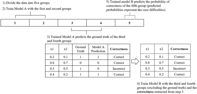
The flow of CDdm. Models A and B are neural networks. × 1 and × 2: example data in the third and fourth groups.
First, data were divided into five sets of equal size. Next, Model A was trained on the first and second sets. Next, the trained model A predicted the cases in the third and fourth sets. Then, Model B was trained with a target variable (Correctness in Fig. 2) defined as whether Model A made correct or incorrect predictions. This allowed model B to predict the probability of correctness from the given data. Lastly, trained Model B made probability predictions of correctness for the fifth set. These predicted probabilities from Model B were the case difficulty of the individual cases in the fifth group. This process was repeated five times to obtain the case difficulties of all sets. Since predicted probabilities have a range between 0 and 1, the case difficulty values also range between 0 and 1, with values closer to 1 indicating more difficult cases.
Models A and B were NNs and Hyperopt was used for hyperparameter tuning. Hyperopt is a Python library for hyperparameter optimization which uses a form of Bayesian optimization to find the best hyperparameter settings16. Hyperopt searched in the following hyperparameter space: learning rate: 0.01, 0.03, 0.1; batch size: 32, 64, 128; number of hidden layers: 1, 2, 3; number of neurons in the hidden layer: 5, 10, 15, 20; and activation function: ReLU, Tanh. Both Models A and B were trained using the Adam optimizer and early stopping with 500 epochs and 50 patience. In Hyperopt, Models A and B were subject to 5 and 10 iterations, respectively, to find the best hyperparameter settings for the simulated data and UCI breast cancer data. For the Telco data and Customer data, since they were larger and more complex than the simulated data, Models A and B were subject to 200 and 200 iterations, respectively, to find the best hyperparameter settings.
CDpu (case difficulty predictive uncertainty)
CDpu defines case difficulty as the variability of predictions made by the model. The main assumption is that easy cases would lead to narrow prediction probability distributions (i.e., less uncertainty) near the correct label. Conversely, difficulty cases would lead to wide prediction probability distributions centered far from the correct label. We used the mean and standard deviation of the prediction probability distribution to calculate the case difficulty. The flow of CDpu is shown in Fig. 3.

The flow of CDpu. \(\mu\): mean value of prediction probabilities; ground truth: the target label of the sample that is excluded in the first step; \(\sigma\): standard deviation of prediction probabilities.
The process began by leaving out one sample as test data (i.e., leave-one-out). The remaining data was divided into 70% for training and 30% for validation, aiming to tune the hyperparameters of a NN. 100 NNs were trained using a randomly shuffled original dataset, excluding the test data. Next, each of the 100 trained NNs generated a prediction probability for the test data. The formula in Fig. 3 was applied to the 100 prediction probabilities and the resulting value represented the case difficulty, with an easy case being closer to 0 and a difficult case being closer to 1.
The formula in Fig. 3 was developed based on the assumption that the worst prediction probability distribution is the uniform distribution. The uniform distribution represents the most conservative uncertainty estimation, and the standard deviation of the uniform distribution can be used as the normalization factor17. Since the prediction probability value ranged between 0 and 1, the standard deviation of the uniform distribution is approximately the square root of one over twelve. When the 100 predicted probabilities formed the distribution, the standard deviation of the prediction probabilities was calculated and divided by the normalization factor. The normalized value was the distribution factor. The distance from ground truth (the location factor) was calculated as the distance between the mean of the prediction probability distribution and ground truth (0 or 1). The average of this distance and the distribution factor became the case difficulty of the test data. For multi-class classification, the distribution and location factors were calculated for each class using the predicted probabilities according to each class. The average of the case difficulty values across all classes became the case difficulty of the test data.
There are rare cases when the case difficulty exceeds 1. This happens when the prediction probabilities exhibit a bimodal distribution pattern for 0 and 1, with two peaks in the distribution. Since the bimodal distribution results in a higher standard deviation than a uniform distribution, it can cause the distribution factor to go over 1. In such instances, the case difficulty is capped at 1.
To reduce computational time, Hyperopt ran under ray tune, which performs distributed hyperparameter tuning18. In Hyperopt, NNs were subject to 100 iterations. To find the best hyperparameter settings, Hyperopt searched in the following hyperparameter space: learning rate: 0.01, 0.03, 0.1; batch size: 32, 64, 128; number of hidden layers: 1, 2, 3; number of neurons in the hidden layer: 5, 10, 15, 20; and activation function: ReLU, Tanh. NN were trained using the Adam optimizer and early stopping with 100 epochs and 30 patience. For the UCI breast cancer data, early stopping was set to 10 patience because of its small sample size.
Evaluation methods and statistical analysis
CDmc, CDdm, and CDpu were assessed using two methods. First, we visually inspected the case difficulty calculated from the existing metrics and proposed metrics. The existing metrics were calculated using the Pyhard Python package18. Second, we computed the Pearson and Spearman correlations between the case difficulty measures from our metrics and the existing metrics in the literature. For example, for a simulated dataset comprising 3000 cases, we obtained 3000 case difficulty values from each of the existing and the proposed metrics. Then, we calculated the Pearson and Spearman correlations between these sets of values. Pearson correlation is a parametric measure of correlation assessing the linear relationship between two continuous variables, whereas Spearman is a non-parametric measure of correlation evaluating the monotonic relationship between two continuous or ordinal variables20. Since we are comparing our metrics with multiple existing metrics that were developed based on various methods to calculate case difficulty, it is uncertain whether the relationship between the case difficulty from our metrics and the existing metrics adheres to parametric (linear) or non-parametric (non-linear or monotonic) patterns. Therefore, we have employed both Pearson and Spearman correlations to investigate the relationships between the metrics. This approach allows us to account for potential linear and non-linear associations and provides a more comprehensive analysis of the relationships.