data
This paper selects parts of China and its surrounding areas as the study area. Research data select his NDVI data from the MODIS (NDVIm) and AVHRR (NDVIa) sensors on Terra and Aqua and his NDVI data from his VIRR (NDVIv) sensors on the Fengyun satellite.31. (I) Compare NDVIv and NDVIa, and NDVIa and NDVIm. (II) comparatively examine the functional relationship between NDVIa and NDVIm, and between NDVIv and NDVIa; (III) NDVIa is used to correct the NDVIv data to levels comparable to NDVIm.
Data used in this study include NDVIa from 1982 to 2015, NDVIm from 2000 to 2019, and NDVIv from 2015 to 2020 (see Table 1). They all have a resolution of 0.05°. This is because there are both NDVIa and NDVIm data for 2005. Therefore, we will compare NDVIa and NDVIm using this year’s data and explore the correlation between the two. Because in 2015 we have both NDVIv data and his NDVIa data. So, using this year’s data, he compared NDVIv and NDVIa to explore the correlation between the two. Finally, we compared his 2019 modified NDVIv with his 2019 NDVIm to validate the success of the model we built.
Figure 1 shows the spectral response function curves of various satellite sensors in the visible and near-infrared spectrum.32. By comparison, it can be seen that the spectral response function of MODIS is narrower than that of AVHRR, and that of AVHRR is narrower than that of VIRR in the visible light band. In the near-infrared band, MODIS has the narrowest spectral response function, followed by HE, VIRR, and AVHRR, the broadest spectral response function. The channels, wavelength ranges, corresponding spectral and sub-satellite resolution information for MODIS, AVHRR, and VIRR sensors are shown in Table 2.

Spectral response function curves of various satellite sensors in the visible and near-infrared spectrum29.
Method
A linear model is a type of machine learning model. Linear models have a relatively simple form and are easy to model. Linear models contain some important basic ideas in machine learning. Many more powerful nonlinear models can be obtained by introducing hierarchies or high-dimensional mappings based on linear models. Linear models come in many forms, with linear regression being a common model. Linear regression learns a linear model to try to predict real-valued output markers as accurately as possible. A loss function is established by establishing a linear model on the dataset, and finally the model parameters are determined with the aim of optimizing the cost function, resulting in a model for subsequent forecasting. A typical linear regression algorithm process is shown in Figure 2.
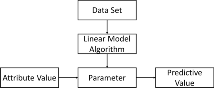
Schematic of the linear regression algorithm flow.
Detailed steps are below33:
-
(I)
Data are normalized and preprocessed. Preprocessing involves cleaning, screening, and organizing the data so that it can be input to machine learning models as feature variables.
-
(Ⅱ)
Different machine learning algorithms are selected to train different datasets, find the optimal machine learning model, and establish a machine learning model based on the normalized vegetation index product obtained by the Fengyun satellite.
-
(III)
Validate and output the long-term series normalized vegetation index of Fengyun satellite.
For 2001-2005, we have both AVHRR NDVI and MODIS NDVI data. So, using these five years of his data, he compared NDVIa and NDVIm and investigated the correlation between the two. Because in 2015 we have both his NDVI data on VIRR and his NDVI data on AVHRR. So, using this year’s data, he compared NDVIv and NDVIa to explore the correlation between the two. Finally, we compared his 2019 modified NDVIv with his 2019 NDVIm to validate the success of the model we built.
A linear machine learning model is used to construct the optimal functional relationship between NDVIa and NDVIm. The formula is as shown in equation (1).
$${\text{Y}}_{{{\text{NDVIm}}}} = \left\{ {{\text{k2}}00{1},{\text{k2}}00{2} , {\text{k2}}00{3}, {\text{k2}}00{4}, {\text{k2}}00{5}, {\text{kmin}}, {\text{kmax }},{\text{kave}}} \right\} \times {\text{X}}_{{{\text{NDVIa}}}} + \left\{ {{\text{m2}}00 {1}, {\text{m2}}00{2}, {\text{m2}}00{3}, {\text{m2}}00{4}, {\text{m2}}00{5 },{\text{mmin}},{\text{mmax}},{\text{mmean}}} \right\}$$
(1)
In the formula, XNDVIa is the NDVI value of AVHRR, YNDVIm is the NDVI value of MODIS, k is the coefficient value of the linear function relationship between NDVIa and NDVIm, k2001, k2002, k2003, k2004, k2005, kmin, kmax, kave are the coefficients of 2001, 2002, 2003, 2004, 2005. , the 5-year minimum, 5-year maximum, and 5-year coefficient mean, respectively. m is the intercept of the linear relationship between NDVIa and NDVIm, m2001, m2002, m2003, m2004, m2005, mmin, mmax, mmean are the intercepts for 2001, 2002, 2003, 2004, 2005, min 5 years, max 55 each Annual, and 5-year average.
Through multiple intercomparison analyses, the best coefficient k and the best coefficient m are selected to determine the best functional relationship between NDVIa and NDVIm.
Based on the above analysis, we continue to build the functional relationship between NDVIa and NDVIv according to equation (2).
$${\text{X}}_{{{\text{NDVIa}}}} = {\text{aZ}}_{{{\text{NDVIv}}}} + {\text{b}}{ .}$$
(2)
In formula (2), Z isNDVIv VIRR, the NDVI value of X.NDVIa is the NDVI value of AVHRR, a is the coefficient value of the linear relationship between NDVIv and NDVIa fitting, and b is the intercept of the linear relationship between NDVIv and NDVIa fitting.
Replace the functional relationship between NDVIa and NDVIv with the optimal NDVIa and NDVIm functional relationship and filter to obtain the refitted NDVIv which is Yvir_ndvi in equation (3). The functional relations for the simulated NDVIv are (3).
$${\text{C}}_{{{\text{NDVIcv}}}} = {\text{k}}_{{{\text{NDVIa}}}} + {\text{m}} = {\text{k}}\left( {{\text{aZ}}_{{{\text{NDVIv}}}} + {\text{b}}} \right) + {\text{m}} = {\text{kaZ}}_{{{\text{NDVIv}}}} + {\text{kb}} + {\text{m}}{.}$$
(3)
In the formula, CNDVI cv is the modified NDVIv(NDVIcv), k is the best fit coefficient of the correlation between NDVIa and NDVIm, and m is the best fit piece of the correlation between NDVIa and NDVIm.
Data for 2005 were selected to compare NDVIm and NDVIa in parts of China and surrounding areas. Data from 2015 were selected to compare his NDVIv and NDVIa in parts of China and surrounding areas. Analysis reveals the correlation between NDVIv, NDVIa, and NDVIm.