Sensory-guided human-machine joint learning accelerates the acquisition of motor imagery brain computer interface control

Participants

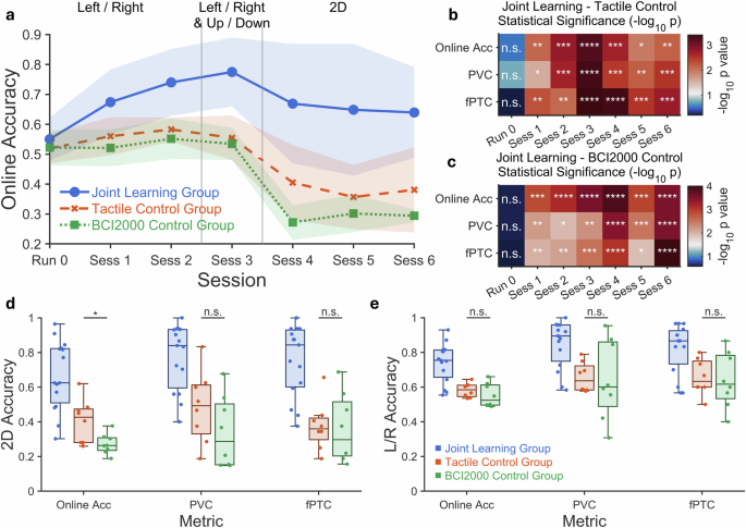
Our study complies with all relevant ethical regulations regarding human research. 31 able-bodied, BCI-naive participants (18 female; mean age 23.8 ± 4.42) were recruited from the Pittsburgh area and provided written informed consent in accordance with the World Medical Association’s Declaration of Helsinki, and according to a protocol approved by the Institutional Review Board of Carnegie Mellon University. Participants were compensated for their time at a rate of $15 per hour. Participants were randomly assigned to three groups: joint learning (n = 15), BCI2000 control (n = 8), and tactile control (n = 8). All participants completed four sessions covering left/right and 2D motor imagery tasks. A subset (n = 21) continued for two additional sessions involving extended 2D control. In addition, an independent EEGNet control group (n = 8) was recruited for an additional control experiment, which followed the same six-session protocol as the other groups.

Tactile stimulation

Tactile feedback was delivered via sustained vibrotactile stimulation using linear resonant actuators (LRAs; 10 mm diameter, VG1040003D, Vybronics Inc.) affixed on the volar aspect of the wrist, near the base of participants’ palm (Fig. 7a). The actuators were driven by a 170 Hz carrier frequency modulated by a 30 Hz sinusoidal envelope, chosen to coincide with the actuator’s resonant peak for optimal efficiency. This waveform was designed to engage both Meissner corpuscles (responsive to 20–50 Hz flutter) and Pacinian corpuscles (responsive to >100 Hz vibration), ensuring broad somatosensory activation^60,61. The palm, densely innervated by both mechanoreceptor types, provided an ideal site for delivering temporally precise tactile cues⁶².

Stimulation was lateralized to the same side as the imagined movement direction (e.g., right-hand stimulation during right-hand MI). In the 2D task, upward movement trials were paired with simultaneous stimulation to both hands, while no stimulation was delivered during downward movement trials. In the joint learning group, tactile stimulation was selectively delivered during “new” trials based on the decoding outcome of the previous trial. In contrast, the tactile control group received identical tactile patterns according to the task instruction, decoupled from user performance. This manipulation enabled the dissociation of sensory reinforcement effects from stimulation alone.

Joint learning framework and sample reweighting algorithm

The proposed sensory-guided joint learning framework facilitates bidirectional co-adaptation between the human user and the machine learning decoder by leveraging two complementary mechanisms: (1) a structured trial paradigm with behavior-contingent tactile stimulation, and (2) a sample-wise reweighting algorithm embedded in the decoder. Together, these mechanisms establish a closed-loop system in which both user and machine continuously adjust based on each other’s learning signals, effectively reducing learning inefficiency from both ends (Fig. 7b).

In motor imagery BCIs, human users often rely on reinforcement-based trial-and-error learning—gradually refining mental strategies based on feedback from system responses and perceived outcomes^26,63. Unlike machines, humans are not gradient-following optimizers; instead, their learning benefits from clear, structured guidance and reward signals. To address this, our framework introduces a pairwise trial structure: in each pair, the first trial is always unstimulated. If this trial is with online accuracy above the threshold, the subsequent trial instructs the participant to reproduce the same motor imagery pattern with a “Copy” instruction, reinforcing internal consistency and promoting neural consolidation. Conversely, if the first trial yields low online accuracy, the second trial is with a “New” instruction—accompanied by tactile stimulation to actively reshape the user’s mental imagery and enhance motor-related signal generation. This structure mimics the logic of error-driven reinforcement learning in biological systems, where correct actions are reinforced, and incorrect ones are redirected via salient cues⁵⁰.

For the decoder, the challenge lies in adapting to dynamically evolving user signals. As users learn and improve, their EEG responses begin to contain increasingly discriminative features—especially during trials reinforced by tactile cues. However, raw training data also contains substantial noise and suboptimal samples, particularly in early learning stages. To handle this, we introduce a sample-wise reweighting algorithm that adaptively adjusts the influence of each training trial based on its loss value. Here, loss refers to how far off the decoder’s prediction is from the correct label, with higher loss indicating poorer classification performance for that sample.

In this algorithm, each sample \({x}_{i}\) corresponds to a 1000 ms EEG window advanced every 40 ms during online decoding, and \({y}_{i}\) denotes its corresponding class label. Before training, EEG samples were bandpass-filtered from 4–40 Hz, downsampled to 100 Hz, and baseline-corrected by subtracting the mean value within the baseline window.

Let \(X={\left\{{x}_{i}\right\}}_{i=1}^{N}\) denote all sliced EEG samples available for decoder training at a given update step, and let \(Y={\left\{{y}_{i}\right\}}_{i=1}^{N}\) denote the corresponding labels. The algorithm first selects an initial reliable subset using a conventional common spatial pattern–linear discriminant analysis (CSP–LDA) pipeline. CSP filters are computed from the available training data pooled across classes, and LDA is used to estimate the posterior class probability for each sample. For each sample \(i\), the confidence score is defined as

The top \({\rho }_{0}\) fraction of samples with the largest \({p}_{i}\) values are selected to form the initial training set \({S}_{0}\), where \({\rho }_{0}\) is the initial inclusion ratio. In the online experiments, ρ₀ was set to 0.2. EEGNet is then initialized on \({S}_{0}\) with uniform sample weights, yielding the initial decoder parameters \({\theta }_{0}\).

The decoder is subsequently refined through iterative reweighting and progressive sample inclusion. At reweighting round \(t\), EEGNet with parameters \({\theta }_{t-1}\) is evaluated on all samples to obtain the per-sample cross-entropy loss:

where \(C\) is the number of classes. \({{\boldsymbol{1}}}\left({y}_{i}=c\right)\) is the indicator function, which equals 1 if the true label \({y}_{i}\) is class \(c\) and 0 otherwise. Here, \({P}_{{\theta }_{t-1}}\left(c,|,{x}_{i}\right)\) is the model-predicted probability for class \(c\), so the loss is the negative log-probability of the true class. The loss values are sorted in ascending order and converted into normalized ranks:

where a smaller rank corresponds to a lower-loss and more reliable sample. The inclusion threshold is progressively increased across reweighting rounds according to

where \(T\) is the total number of reweighting rounds. In the online experiments, \(T\) was set to 9. The corresponding number of included samples at round \(t\) is \({M}_{t}=\left\lfloor {\rho }_{t}N\right\rfloor\), where \(\left\lfloor .\right\rfloor\) denotes rounding down to the nearest integer.

Each sample is then assigned a weight according to its normalized loss rank:

Thus, samples with lower loss receive larger weights, whereas samples outside the current inclusion threshold are excluded from that reweighting round. The final weights are normalized to [0, 1] for numerical stability. The updated training set is defined as

EEGNet is fine-tuned on \({S}_{t}\) by minimizing the weighted objective:

This procedure is repeated for \(T\) rounds, yielding the final decoder parameters \({\theta }^{*}={\theta }_{T}\) and the final sample weights \(v={v}^{(T)}\). A step-by-step pseudocode implementation is provided in Supplementary Table 1, with an illustrative schematic in Supplementary Fig. 15.

The decoder update was performed once after each training run. During each online run, decoder parameters were fixed, and no within-run model updating was performed. The updated decoder was then used in the subsequent run. No decoder fine-tuning was performed during online test runs. This update schedule synchronized user learning and decoder adaptation across two coupled timescales. At the trial-pair level, the participant’s online performance determined the subsequent copy/new instruction and whether tactile stimulation was delivered, thereby guiding the user’s exploration or consolidation of motor imagery strategies while the decoder remained fixed. At the run level, the EEG samples generated under this trial policy were then used for decoder updating through the sample reweighting algorithm. In this way, user-side learning and machine-side adaptation are coupled through the evolving separability of the EEG samples.

This mechanism assigns greater importance to trials that already contain reliable or behaviorally reinforced neural patterns—including those enhanced through tactile stimulation—while down-weighting noisy or misaligned samples. Because reinforced trials tend to produce lower losses, the windows belonging to these trials naturally receive higher weights and exert greater influence on subsequent parameter updates. As user learning progressively shapes the underlying neural representations (e.g., stronger or more consistent ERD/ERS patterns), the reweighting process amplifies the decoder’s sensitivity to these emerging structures. In this way, human learning directly guides machine adaptation, creating a synchronized co-learning process. The progressively increasing inclusion threshold implements a curriculum-style progression inspired by curriculum and self-paced learning paradigms^64,65, in which optimization begins with highly reliable samples and gradually incorporates more challenging ones, improving convergence stability and robustness.

Crucially, the decoder’s output also serves as feedback to the user through the online cursor and the copy/new trial structure. The updated decoder, therefore, influences the feedback available in subsequent runs, which in turn shapes the user’s future motor imagery strategies. This establishes a closed-loop co-learning cycle in which users learn to generate more separable neural patterns and the decoder progressively prioritizes those patterns during optimization.

This synergistic alignment is illustrated in Fig. 7c. In traditional systems, user learning trajectories (orange arrow) often diverge from the global loss gradient due to unguided exploration. In contrast, the joint learning paradigm integrates tactile guidance and selective feedback (blue arrow) to better align the subject’s learning path with the optimal descent direction (dashed line), thereby achieving more efficient convergence toward the global optimum.

Experimental paradigm and BCI protocol

Each experimental session comprised a series of discrete motor imagery (MI) trials. Participants were seated in front of a computer monitor, wearing a 64-channel EEG cap (Neuroscan Quik-Cap) with their palms resting on tactile actuators positioned beneath each hand (Fig. 7a). EEG signals were recorded using SynAmps 2/RT amplifiers (Compumedics Neuroscan), with electrodes arranged in a modified international 10–20 layout, placing the reference electrode centrally between Cz and CPz. Impedances were reduced below 5 kΩ prior to each session. EEG data were sampled at 1000 Hz and notch-filtered at 60 Hz to eliminate power line interference. The digitized signals were streamed to the BCI2000 platform in 40 ms packets for real-time signal processing and BCI control.

All participants initially completed a BCI2000-based calibration run using a left/right MI task to establish baseline decoding accuracy. They then participated in 4 to 6 sessions. The first two sessions involved left/right MI tasks only, the third session introduced a combination of left/right and up/down targets, and the remaining sessions involved full 2D control. Each session comprised six runs: (1) a calibration run without feedback, (2) a test run with visual feedback but no tactile stimulation, (3–5) three training runs using the assigned paradigm, and (6) a post-training test run. A 5-min rest was provided prior to the final run. Test runs included half the number of trials as calibration and training runs (60/30 for L/R and 64/32 for 2D; see Supplementary Fig. 14a, b for trial details).

Each MI trial followed a fixed structure. A central fixation appeared for 2 s, followed by a directional cue indicating the MI target. Participants performed kinesthetic imagery of the corresponding limb with the cursor feedback for 5 s, followed by a 2 s rest (Supplementary Fig. 14c). Left/right cues instructed participants to imagine left or right hand movement to move the cursor horizontally. For upward movement, participants were instructed to imagine simultaneous bilateral hand movement. Downward movement corresponded to resting and not performing MI. Visual cursor feedback was provided during all runs except calibration.

In the joint learning group, trials were organized in pairwise structures, with each pair sharing the same directional cue. If the first trial of a pair achieved online accuracy above a pre-defined threshold, the second trial displayed the “copy” instruction along with the direction cue, prompting the participant to replicate the same mental strategy. If the first trial fell below the threshold, the second trial displayed the “new” instruction and delivered tactile stimulation to the corresponding hand.

In the tactile control group, trials were also presented in direction-matched pairs. However, no “copy/new” cues were provided. Instead, tactile stimulation was delivered in every trial, regardless of prior performance. This design isolated the effects of tactile enhancement without contingent reinforcement or strategic feedback.

The BCI2000 control group received no tactile stimulation or strategic cues across all runs. The number of trials and session structures were identical to those in the joint learning group, enabling direct comparison of learning outcomes under passive decoder conditions. For long-term experiments, the BCI2000 control group received feedback calculated by EEGNet, using the same EEGNet configuration as that used in the tactile control group and the EEGNet control group.

In the EEGNet control group, trials were presented in a non-pairwise, randomized order, with no tactile stimulation or “copy/new” instructional cues. Decoder outputs were generated using the same run-wise update schedule as in the joint learning and tactile control group. This additional control condition was designed to isolate the influence of decoder architecture and adaptation from the sensory-guided joint learning framework by removing tactile reinforcement and pairwise strategic structure while preserving the EEGNet decoder.

For training parameters of the EEGNet, model optimization was performed using mini-batch stochastic gradient descent with the Adam optimizer. The initial learning rate was set to 1 × 10⁻³, with default momentum parameters (β₁ = 0.9, β₂ = 0.999). Binary cross-entropy loss was used as the base objective for classification. Training was conducted for a maximum of 300 epochs with early stopping based on training loss convergence to prevent overfitting. For subsequent sessions, weights were initialized from the model trained in the immediately preceding session, enabling gradual decoder adaptation over time. In contrast, for the long-term experiments, both the weighted EEGNet and the conventional EEGNet were reinitialized and trained from scratch in each session, without carrying over weights from previous sessions. No online fine-tuning was performed during test runs; all model updates occurred offline between runs.

For parameters of online experiments in Supplementary Table 1, \({Init}\) was set as 0.2 and \(T\) set as 9. A fixed accuracy threshold of 70% was used across all participants. This value was selected a priori based on established conventions in the BCI literature, where approximately 70% classification accuracy is commonly considered indicative of reliable and usable BCI control^10,66. Applying a uniform threshold across participants ensured consistency of the training protocol and avoided subject-specific tuning that could confound group-level comparisons.

Performance metrics and analysis methods

To quantify both BCI control performance and the underlying learning processes, we employed a combination of behavioral, algorithmic, and neurophysiological metrics. Online accuracy, the primary behavioral metric, was computed for each trial as the mean classification accuracy across all 1000 ms sliding windows (stepped by 40 ms) within the 5 s motor imagery period, which is a common metric for continuous tasks^29,66,67. At each window, the classifier output determined whether the cursor moved toward the cued target direction; the online accuracy was then calculated as the proportion of correct movements over the total number of movements in that trial. This method has two advantages: the chance level is analytically defined as \(1/{N}_{{classes}}\),where \({N}_{{classes}}\) is the number of possible target directions; and it produces a continuous accuracy score for each trial, enabling fine-grained comparisons between trials.

To complement this continuous measure, we also employed two discrete, run-level performance metrics widely used in BCI2000-based experiments⁴². The percent valid correct (PVC) was defined as:

where a hit denotes the cursor reaching the correct target at the end of the trial, and a miss denotes the cursor hitting an incorrect target. Trials in which the cursor did not reach any target were classified as aborts and excluded from the PVC computation.

The forced percent total correct (fPTC) extended this metric by assigning abort trials to the spatially closest target (either correct or incorrect) before recomputing the hit/miss counts:

where \({N}_{{Trial}}\) stands for the number of trials in the run^68,69,70. Like online accuracy, the chance level for PVC and fPTC is \(1/{N}_{{classes}}\), but these discrete measures directly reflect the proportion of successfully completed trials, providing a more task-completion–oriented performance assessment.

The system performance was further assessed using an online test loss. Rather than reflecting training dynamics, this metric quantifies how well the decoder generalizes to unseen streaming data during online operation. Specifically, we computed the mean cross-entropy loss over all prediction windows within a run, using the continuously acquired EEG signals as test input (see Supplementary Methods 1). A lower online test loss indicates both improved decoders fitting to the participant’s evolving neural patterns and reduced ambiguity in the extracted features. Tracking this loss across runs, therefore, captures the combined learning effects of both the human user and the adaptive algorithm.

To quantify co-adaptation between the user and the decoder, we employed a vector-based alignment metric across consecutive training runs. For each subject and session, we computed the signal change vector as the difference in average neural signal vectors between two successive runs. In parallel, we obtained the averaged decoder gradient vector by feeding the neural signal from the earlier run into the trained network. The alignment between these two vectors was then characterized using projection length (magnitude of the dot product) and cosine similarity, reflecting not only the directional agreement but also the extent to which neural changes aligned with the model’s most informative dimensions (see Supplementary Methods 2). To visualize the adaptation process, neural features were reduced to two dimensions using Principal Component Analysis (PCA) and plotted sequentially across runs, allowing the evolution of neural representations to be tracked over time.

For neurophysiological analysis, event-related desynchronization/synchronization (ERD/ERS) and event-related spectral perturbation (ERSP) were quantified in the alpha (8–13 Hz) and beta (13–30 Hz) frequency bands from electrodes C3 and C4. Continuous EEG data were segmented into epochs and transformed into the time–frequency domain using a complex Morlet wavelet transform, yielding spectral power estimates at each time–frequency point.

ERD was expressed as the percent change relative to its baseline proceeding task window⁵⁵, calculated as:

where P(t,f) is the spectral power at time \(t\) and frequency \(f\).

ERSP was computed as the relative power change in decibels (dB)⁷¹, defined as:

where \({P}_{{Baseline}}(f)\) refers to the average baseline power at frequency \(f\). ERSP values are thus reported in decibels (dB), enabling direct interpretation of spectral power increases (positive values) or decreases (negative values) relative to baseline.

To interpret the learned features of the neural network models, we employed activation and gradient-weighted class activation mapping (Grad-CAM)^72,73. Activation refers to the weighted sum of the input values and their corresponding network weights, representing how strongly a given feature contributes to a neuron’s response. While Grad-CAM highlights the spatial and spectral regions most influential for the decoder’s decision. In our implementation, Grad-CAM was computed from the gradients of class scores with respect to convolutional feature maps, and visualized on the EEG topography to reveal physiologically meaningful features. A full description of the equations and derivations of the procedure is provided in Supplementary Fig. 16, Supplementary Methods 3.

For each trained model, the gradient of the class score with respect to the feature maps of the final convolutional layer was computed. Specifically, for each convolutional kernel \(k\), the gradient \(\frac{\partial {y}^{c}}{\partial {A}^{k}}\) was averaged spatially to obtain importance weights \({a}_{k}^{c}\). The Grad-CAM map for class c was then calculated as:

Where \({A}^{k}\) denotes the feature map of kernel \(k\) and \({a}_{k}^{c}\) reflects its contribution to class \(c\). ReLU (rectified linear unit) is an activation function defined as \({ReLU}\left(x\right)=\max (0,x)\), which retains positive responses and sets negative ones to zero, thereby preserving strong feature activations while suppressing noise⁷⁴. The resulting Grad-CAM maps were interpolated to the EEG channel layout, yielding topographical visualizations of feature relevance. For the frequency-domain, Grad-CAM values were aggregated across kernels with center frequencies in each band, and normalized to quantify the relative importance of frequency ranges. For the spatial Grad-CAM, Grad-CAM maps were averaged across classes to reveal overall activation patterns, reflecting the consistent and robust neural features captured by the model. These maps highlight the cortical regions and spectral bands most influential for the model’s decision, providing an interpretable link between neural dynamics and decoder learning.

All EEG preprocessing and decoder analyses were performed in Python, while behavioral metrics and ERD analyses were conducted in MATLAB and EEGLAB⁷⁵.

Statistical analysis

All statistical analyses were performed in MATLAB R2024b (MathWorks, USA). Data are reported as mean ± s.e.m. or s.d., as specified in the figure legends. Given the relatively modest sample sizes, formal normality tests were not employed, as such tests have limited statistical power under small-sample conditions. Instead, non-parametric tests were adopted as a conservative default for single-factor and pairwise comparisons.

For comparisons involving one factor or pairwise contrasts, we used Wilcoxon-based non-parametric tests (signed-rank or rank-sum, as appropriate). Effect sizes for all non-parametric comparisons were quantified using the rank-based effect size r, computed as

where Z denotes the standardized test statistic and N the number of observations used in the corresponding test. This measure provides a distribution-free estimate of effect magnitude and is applicable to both paired and unpaired non-parametric comparisons.

For analyses involving multiple factors or repeated measurements across conditions or sessions, one-way or two-way repeated-measures ANOVAs were employed, with primary interest placed on interaction effects (e.g., group × session). Partial eta squared (ηp²) was reported as the effect size for ANOVA results. Greenhouse–Geisser correction was applied when the sphericity assumption was violated.

To assess sample size adequacy for the primary learning-related effects, we additionally conducted a simulation-based power analysis tailored to the non-parametric statistical framework used in this study. Statistical power was estimated via Monte Carlo simulations based on the empirical data distributions observed across training sessions, rather than relying on parametric assumptions.

This combined approach allowed conservative inference for simple comparisons while preserving statistical interpretability for multi-factor learning effects. Post hoc pairwise tests were corrected for multiple comparisons using the Bonferroni method. Statistical significance was set at p < 0.05 unless otherwise noted.

Ethics

Every experiment involving human participants has been carried out following a protocol approved by the Institutional Review Board of Carnegie Mellon University. Each participant gave informed written consent.

Reporting summary

Further information on research design is available in the Nature Portfolio Reporting Summary linked to this article.