Microseismic monitoring with the quake neural operator

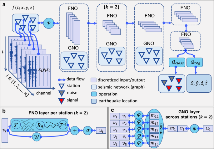
We propose QNO, a multi-task neural operator designed for earthquake detection and location directly on continuous seismic waveform data without explicit phase picking or phase association. This section provides an overview of the QNO, including its architecture, loss function, and training dataset.

Quake neural operator in multi-task learning

QNO performs a nonlinear mapping from the input function f(t; x, y, z) to the output in a multi-task learning framework. It consists of a shared feature extractor \({{\mathcal{F}}}\) followed by separate classification \({{{\mathcal{Q}}}}_{{{\rm{class}}}}\) and regression \({{{\mathcal{Q}}}}_{{{\rm{reg}}}}\) branches:

where h represents the shared feature extracted from the input function with a nonlinear operator \({{\mathcal{F}}}\). \({{\mathcal{G}}}\) denotes the QNO. For multi-station seismic data, (x, y, z) denotes the spatial coordinates of the seismic stations, while t denotes the temporal coordinate. The input samples are the discretized values of this function f(t; x, y, z) in both space and time. In principle, neural operators \({{\mathcal{F}}}\), \({{\mathcal{G}}}\), \({{{\mathcal{Q}}}}_{{{\rm{class}}}}\) and \({{{\mathcal{Q}}}}_{{{\rm{reg}}}}\) are formulated to operate on inputs defined on arbitrary discretizations⁵⁹. In practice, this allows QNO to be trained and evaluated on varying seismic network geometries.

For earthquake detection, the classification task \({{{\mathcal{Q}}}}_{{{\rm{class}}}}\) processes the shared representation h to produce a spatial logits field, which is converted into a probability function p(x, y, z) using the softmax function:

The probability function is evaluated at the station locations. Here, \({{\bf{p}}}={\{{{{\bf{p}}}}_{i}\}}_{i=1}^{n}\in {{\mathbb{R}}}^{n\times 2}\) denotes the probabilities for earthquake signals and noise at stations located at (x_i, y_i, z_i), where i ∈ {1, 2, …, n} and n is the number of stations in the input. Each \({{{\bf{p}}}}_{i}\in {{\mathbb{R}}}^{2}\) represents the probability distribution over signal and noise for the i-th station:

For earthquake location, the regression task outputs the earthquake source location \((\widehat{x},\widehat{y},\widehat{z})\) and origin time \(\widehat{t}\):

where \(\widehat{{{\bf{r}}}}=(\widehat{x},\widehat{y},\widehat{z},\widehat{t})\in {{\mathbb{R}}}^{4}\) is the predicted result.

Architecture of quake neural operator

The architecture of QNO (Fig. 1) mainly relies on two types of neural operators, which can efficiently process the spatiotemporal representation of seismic data over time and space (see Supplementary Note 1): One is the Fourier Neural Operator (FNO)⁵⁶ and the other is the Graph Neural Operator (GNO)⁵⁷. FNO learns global correlations in the temporal axis using Fourier transforms, effectively capturing long-range dependencies in the data. GNO operates on graph structures to model relationships among seismic stations, which effectively deals with the irregular sampling of seismic data in the spatial domain. Started from the input function f(t; x, y, z), the neural operator \({{\mathcal{F}}}\) shared by both the classification and regression tasks can be viewed as a series of mappings through layers of operation:

where \({\circ }\) denotes the mapping between two layers. With k = 3, QNO uses three combinations of layers of FNO and GNO. The input function is first passed through an up-projection layer \({{\mathcal{P}}}\), which maps the input function to a high-dimensional representation. Then the up-projected data is passed through three combinations of FNO and GNO layers, allowing sufficient exchange of information between the time and space domains.

Each FNO layer performs a 1-D spectral convolution along the temporal axis at each station: we apply a Fourier transform to the per-station features, multiply the lowest M_k frequency modes by learned complex weights while zeroing higher modes, inverse-transform back to the time domain, and then combine the result with a pointwise (1 × 1) linear projection, followed by a nonlinearity⁵⁶. To reduce boundary artifacts associated with applying Fourier transforms to non-periodic time series, we apply zero-padding (50 samples on each end) prior to the FNO layers. This suppresses spurious high-frequency components induced by discontinuities at the signal boundaries and stabilizes the spectral representation used by the operator layers. In addition, each FNO layer retains only the first M_k lowest-frequency modes, as high-frequency components are more difficult to learn and are truncated during training⁵⁶. The number of modes in each FNO layer is 24, 12, 8, 8, and 8, respectively. The width (or channel number) of the discretized function at each station varies with the dimension. Across the FNO layers, the per-station discretized representation \(v(t;{{{\bf{x}}}}_{i})\in {{\mathbb{R}}}^{{C}_{k}\times {T}_{k}}\), with x_i = (x_i, y_i, z_i), takes the following shapes by layer: 48 × 1500, 96 × 500, 192 × 100, 192 × 50, and 24 × 50. The first dimension is the channel width C_k; the second is the number of time samples T_k. As the network progresses through downsampling, the number of Fourier modes M_k is reduced in proportion to the compressed resolution, while the channel dimensions are increased to enrich feature representations. Nonlinearity is introduced in all FNO layers using the Gaussian Error Linear Unit⁶⁴, which applies a smooth, probabilistic gating mechanism that approximates the input multiplied by the cumulative distribution function of a standard normal distribution. The output of the last FNO layer is flattened into 1200 channels before feeding into \({{{\mathcal{Q}}}}_{{{\rm{class}}}}\) and \({{{\mathcal{Q}}}}_{{{\rm{reg}}}}\).

At each GNO layer, stations are treated as nodes in a graph, and their features are updated through a message-passing framework⁶⁵. The graph is constructed in the input spatial domain using a distance threshold D (two stations are connected with an edge if their pairwise distance ≤D). Unless otherwise noted, for example, when explicitly analyzing generalization with respect to D (see Supplementary Fig. 30), we set D = 40 km. Per-station temporal features \(v(t;{{{\bf{x}}}}_{i})\in {{\mathbb{R}}}^{{C}_{k}\times T_{k}}\) produced by the preceding FNO layer serve as node features. For each edge (i, j), an edge message is computed by a differentiable map φ that takes the two node features concatenated along the temporal axis as the input, \({m}_{ij}=\varphi \,\left(v({{{\bf{x}}}}_{i}),v({{{\bf{x}}}}_{j})\right)\). Node i then performs mean aggregation \({\bar{m}}_{i}=\frac{1}{| {{\mathcal{N}}}({{{\bf{x}}}}_{i})| }{\sum }_{j\in {{\mathcal{N}}}({{{\bf{x}}}}_{i})}{m}_{ij}\) and updates its representation via a second map ψ: \(u({{{\bf{x}}}}_{i})=\psi \,\left(v({{{\bf{x}}}}_{i}),{\bar{m}}_{i}\right)\). In QNO, both φ and ψ are two-layer MLPs with hidden width 4C_k, where C_k is the channel dimension of the node features output by the k-th FNO layer preceding the k-th GNO layer. The message-passing framework in the GNO layer is permutation-invariant, accommodates irregular station layouts, and couples spatial communication with the temporal representations learned by the FNO. QNO uses three GNO layers interleaved with FNO layers.

The final output h from the shared part branches into two separate parts for classification and regression, respectively. To reduce the dimensionality of the shared feature representation h, we use two different down-projection layers for the separated branches of the regression and classification tasks. The classification output is generated by passing h through the down projection layer \({{{\mathcal{Q}}}}_{{{\rm{class}}}}\) and applying the softmax function. The regression output is generated by passing h through the down-projection layer \({{{\mathcal{Q}}}}_{{{\rm{reg}}}}\), producing the predicted earthquake source location and origin time. Both \({{{\mathcal{Q}}}}_{{{\rm{class}}}}\) and \({{{\mathcal{Q}}}}_{{{\rm{reg}}}}\) are two-layer fully connected neural networks.

Loss function for the multi-task learning framework

The total loss function of the multi-task neural operator is a weighted sum of the individual task losses:

where α is a weight that balances the contribution of the regression task relative to the classification task. \({{{\mathcal{L}}}}_{{{\rm{class}}}}\) is the classification loss; and \({{{\mathcal{L}}}}_{{{\rm{reg}}}}\) is the regression loss. Here we choose α = 1.

The cross-entropy loss function for the classification task is an expectation over the joint distribution \((X,Y) \sim {{{\mathcal{D}}}}_{1}\), where X denotes evaluations of the seismic wavefield function f(t; x, y, z) at the station locations of a seismic network, and Y = [Y^signal, Y^noise] denotes the corresponding labels:

The regression task uses mean squared error (MSE) to predict the source parameters of an earthquake \(\widehat{{{\bf{r}}}}=(\widehat{x},\widehat{y},\widehat{z},\widehat{t})\):

where r_true = (x_true, y_true, z_true, t_true) contains the ground-truth earthquake source locations and origin times. These labels usually come from an existing earthquake catalog used to construct the training dataset.

Training dataset

We use a training dataset previously employed to train two deep neural phase pickers, PhaseNet¹¹ and PhaseNO¹⁹. Using a similar training dataset enables a fair comparison and evaluation of the performance of each method after training. The dataset consists of three-component earthquake waveforms and event catalogs spanning 30 years from the Northern California Earthquake Data Center (NCEDC). To train QNO for microseismic monitoring, we focus on events with magnitudes up to 2. To improve accuracy and minimize uncertainties, we select events recorded by at least eight stations. The event depths range from -4 to 36 km (Fig. 2). Depths are referenced to sea level; negative values indicate earthquakes occurring above sea level in high-elevation regions (e.g., mountains in California).

We adopt a temporal split as the primary setting: events prior to 2016 form the training set, while events from 2016 and 2017-2021 are designated as the validation and test sets, respectively. This selection yields 7972 events in the training set, 1402 events in the validation set, and 1019 events in the test set. This design reflects practical deployment, where models trained on historical earthquakes are applied to future events; following common practice, this temporal split implicitly disregards the question of stationarity. It also introduces temporal distribution shift due to changes in station coverage, noise, and catalog completeness. Unless otherwise specified, all evaluations use the model trained on events before 2016. For a complementary random split and additional analyses, see Supplementary Note 4 and Supplementary Figs. 4 and 5.

We perform data augmentation and pre-processing when preparing the training dataset. In the NCEDC dataset downloaded from the data center, waveforms from all stations associated with an event contain earthquake signals. However, in real-world scenarios, not all stations record earthquake waveforms. To simulate this, we generate up to 16 virtual stations with random locations within the computational domain and assign noise waveforms to these virtual stations. Each station is assigned a classification label: [1, 0] for earthquake signals and [0, 1] for noise, where the first channel indicates \({p}_{i}^{signal}\) and the second channel represents \({p}_{i}^{noise}\). To improve QNO’s ability to detect events in the presence of strong noise, we also added noise to the earthquake waveforms at real stations. The noise waveforms were randomly selected from the 235,000 noise samples available in the STEAD dataset⁵⁸, and the noise varies across different stations. Then these raw waveforms were first preprocessed by removing the trend using a demeaning procedure and applying a bandpass filter with a frequency range of 1 to 10 Hz. After filtering, the waveforms were normalized by dividing each channel by its maximum value.

We use a relatively short time window of 15 s to train QNO. This window length is appropriate for local microseismic monitoring where waves decay fast during propagation. A short time also reduces the possibility of the existence of multiple events in one sample. Since QNO faces the challenge of handling multiple events within a single input time window (see Supplementary Note 3), selecting a short time window is a straightforward way to address this issue and is particularly effective for microseismic monitoring, where inter-event times are generally much longer than those in aftershock sequences of large earthquakes. Moreover, we use overlapping time windows when processing continuous data, which helps to reduce the possibility of missing events.

We construct a computational domain that can cover the locations of the local earthquake and stations for each sample in the dataset. Coordinates on the computational domain have values between 0 and 1, which is favorable for the learning process. The physical lower bounds of longitude λ₀ and latitude ϕ₀ for the computational domain are given by:

where λ_max is the maximum longitude, \({\lambda }_{\min }\), the minimum longitude, ϕ_max, the maximum latitude, \({\phi }_{\min }\), the minimum latitude of all stations around an earthquake. Each sample is mapped with a varying center so that all stations in the graph are around the middle of the computational domain. In addition, d represents the extent of the computational domain on the Earth’s surface. The chosen range d should be large enough to encompass all the stations within the graph. Since the propagation range of small-scale events is typically short, a selection of d = 1. 2° is sufficient and appropriate for monitoring local earthquakes in our experiments. After determining the physical lower bounds of the computational domain, we can calculate the relative position of each station within this domain:

where λ_i, ϕ_i, and η_i are respectively the longitude, latitude, and depth of the i-th station. η_max is the maximum depth and \({\eta }_{\min }\) is the minimum depth of the computational domain. We choose \({\eta }_{\min }=-4\) km and η_max = 36 km to include the depth of all earthquakes in the dataset. The computational domain and the relative positions (x_i, y_i, z_i) of the stations are computed independently for each data sample during training. For real-world scenarios, the relative positions are computed only once for a given seismic network. These transformed coordinates are treated as node attributes and three additional channels of the input, along with the three-component waveform information.

Similarly, the regression label for earthquake location is the earthquake’s relative location (x_true, y_true, z_true) in the computational domain:

where (Λ, Φ, H) denotes the ground-truth earthquake location, which in practice is usually taken from the earthquake catalog. The time predicted by QNO is the occurrence time of an event relative to the start of the input time series. Assuming the origin time T is within a range of 10 s earlier (t_min = − 10 s) and 10 s later (t_max = 10 s) than the starting time of an input waveform, the time t_true of the regression label that we train QNO to predict should be:

We train QNO with the Adaptive Moment Estimation (Adam) optimizer⁶⁶ with a batch size of one and a learning rate of 10⁻⁴. Adam is a stochastic gradient-based optimizer that computes adaptive learning rates for each parameter based on estimates of first and second moments of the gradients. The training takes around three hours for one epoch on one NVIDIA Tesla V100 GPU. We train the model with 19 epochs and then evaluate it on the test dataset and 10-day continuous data from the Geysers geothermal field.

When evaluating performance on the test dataset (Fig. 4), we first convert the predicted coordinates \((\widehat{x},\widehat{y},\widehat{z},\widehat{t})\) of each sample to physical coordinates corresponding to longitude, latitude, depth, and origin time. We then compute the differences between the converted predictions and the corresponding catalog values (Λ, Φ, H, T). Location errors in degrees are converted to kilometers using a factor of 111 km/° for latitude and approximately 88 km/° for longitude, based on the mean latitude of the study area.