Principled approaches for extending neural architectures to function spaces for operator learning

In the past decade, deep learning has led to unprecedented advances in domains such as computer vision, speech and natural language processing. Following this success, deep learning is poised to have an arguably even greater transformational impact on the natural sciences. Although underlying data in all these areas come in vastly different structures, the standard models powering deep learning, neural networks, consume processed versions of data in the form of finite-dimensional vectors (for example, pixel representations of images and videos, word embeddings of language or measurements of physical systems).

Yet, many physical phenomena of interest are inherently captured by continuum descriptions: quantities in fluid dynamics and thermodynamics, continuum mechanics or electromagnetism depend on continuous spatiotemporal variables and are often governed by partial differential equations (PDEs), where the central task is to map an input function, such as coefficients or forcing terms, to a solution function. Common tasks in computer vision can be viewed similarly: natural scenes or objects can be idealized as functions of space and time, whereas images and videos are finite-resolution discretizations of underlying functions.

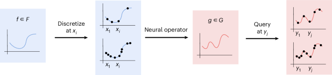
Although classical neural networks can process discretizations of continuous quantities (for example, on a mesh or grid), they typically either rely on a fixed discretization or do not generalize to unseen resolutions. However, we would like the learned map to be discretization agnostic with respect to the specific choice of discretization and its resolution (up to a vanishing discretization error). Furthermore, in numerous applications, it is essential for the output to be a function that can be queried at arbitrary coordinates, enabling further downstream operations (for example, differentiation and integration). To this end, neural networks have recently been generalized to neural operators, which are naturally formulated to operate on functions rather than vectors (Fig. 1). The empirical neural operator is evaluated on samples, but its parameters describe a function-space map: by construction, it outputs functions or empirical evaluations of functions that can be queried at arbitrary coordinates and that are consistent across different discretizations of the input function (more precisely the outputs only differ by a discretization error that vanishes as the discretization is refined). This property of being agnostic to the underlying discretization enables learning of function-to-function mappings and multiscale phenomena for the wide range of tasks where the underlying data are captured by continuum descriptions. These properties have led to substantially improved performance and generalization, as well as powerful capabilities, such as zero-shot super-resolution, in a series of practical applications. Supplementary Sections A.2, A.3 and A.5 formalize the empirical evaluation of neural operators on discretized inputs, define discretization convergence and relate discretization, approximation and optimization errors to zero-shot prediction across resolutions.

**Fig. 1: Illustration of a neural operator.**

Using neural networks to represent continuous functions, known as implicit neural representations or neural fields, has a long history¹. Special cases include physics-informed neural networks², where the neural network approximates a PDE solution function by optimizing its parameters to reduce deviations from the governing equations. Shortly after the introduction of neural operators, three-dimensional scenes in graphics and computer vision have been similarly represented using neural radiance fields^3,4,5. In both of these cases, the neural network represents a single function, that is, a single PDE solution or three-dimensional scene. By contrast, neural operators can be viewed as generalizations of neural fields because they output a function for any given input function, that is, they can learn operators that act on functions. Neural operators can be viewed as conditional neural fields⁶, where the conditioning variable is the input function. Alternatively, one can condition the implicit neural representations on the parameters of a finite-dimensional parametrization of the space of input functions^7,8. Although this can be viewed as a special case of an encoder–decoder neural operator (Supplementary Section B.6), neural operators are more general and can handle input and output functions based on point evaluations without the need for parametrizations.

In this Article, we present how neural network layers can often be extended to function spaces by identifying the continuous operator that the finite-dimensional layer discretizes. Once that operator has been identified, the layer can be discretized in a way that respects the coordinates, quadrature weights and sampling structure of the underlying function, rather than only the index set of a particular array.

We first describe the operator-learning setting and the principles that make neural operators discretization agnostic. We then give a general recipe for converting neural network layers into operator layers, summarize the resulting correspondences for fully connected layers, pointwise maps, convolutions, graph neural networks, transformers and encoder–decoder architectures and finally evaluate these distinctions empirically.

From discrete to continuous learning on function spaces

Classical neural networks aim to approximate functions

$$x\longmapsto f(x)$$

(1)

between (finite-dimensional) Euclidean spaces, such as ${{\mathbb{R}}}^{{d}}$. More precisely, they take a vector x as input and output another vector f(x). By contrast, we want to construct operators

between (infinite-dimensional) function spaces, such as continuous functions. We use ${\mathcal{F}}$ and ${\mathcal{G}}$ to denote the function spaces for the input and output functions, which are typically suitable subspaces of continuous functions. Operators take a function f as input and output another function g (see Table 1 for a comparison and Supplementary Section A.1 for details on notation).

Table 1 Notation and comparison of neural networks to neural operators

The transition from discrete to continuous problems requires a change in how we represent and manipulate data. Although we are interested in learning mappings between functions, we typically do not have access to the actual functions numerically. Instead, neural operators are designed to work on a discretization${(({x}_{i},f({x}_{i})))}_{i=1}^{n}$ of a function f, assuming that we observe the function on a set of points x_i (that is, a point cloud or grid; see Supplementary Section A.1 for alternative representations). Moreover, the output of the neural operator, a function g, can be queried at arbitrary coordinates y in its domain (see Fig. 1 for an illustration).

A map learned directly between two arrays at one resolution need not define a consistent map between the underlying functions. If the parameters, receptive field, aggregation rule or tokenization are tied to input indices rather than domain coordinates, changing the discretization changes the operation applied. The goal is therefore not merely to accept arrays of varying sizes but to ensure that these arrays are all discretizations of the same underlying function-space map.

We now formulate a collection of practical principles for the design of neural operators to guide their effective use in scientific machine learning.

Defining principles of neural operators

To learn a mapping between functions in practice, the following properties should be satisfied:

Discretization agnostic: the learned mapping should be applicable to functions given at any discretization and produce consistent outputs across resolutions.
Fixed number of parameters: the number of learnable parameters needs to be fixed and independent of the discretization.
Universal approximation: the family of mappings should be able to (provably) approximate, with arbitrarily low error, any sufficiently regular operator.

Neural operators represent a principled extension of neural networks to function spaces designed from first principles to satisfy these properties. They are parametrized by a finite number of learnable parameters, universally approximate sufficiently regular function-to-function mappings and provide consistent predictions across resolutions. In practice, neural operators still operate on discretized functions but also respect the underlying functions they model and are not tied architecturally to a fixed set of observation points. In particular, their outputs are functions that can be evaluated on arbitrary discretizations, and the outputs of a neural operator for different discretizations only differ by a discretization error that can be made arbitrarily small by refining the discretization, in which case we say that the neural operator is discretization convergent (Supplementary Section A.3).

Features of neural operators

Neural operators provide a principled framework to learn mappings on functional data, and their ability to train and test on data with varying discretizations unlocks unique features and advantages:

Canonical function-space formulation: for many tasks, the ground truth mapping is naturally an operator, that is, a mapping between functions. If we train a neural network that is not discretization agnostic, we can overfit to the training discretization(s). Operator learning allows us to approximate the ground truth operator and establish rigorous theoretical guarantees (Supplementary Section A.5). In addition, having output functions that can be queried arbitrarily is useful for downstream applications that require derived quantities such as derivatives or integrals.
Data efficiency: standard numerical solvers often create their meshes adaptively, which naturally leads to datasets with different discretizations^9,10,11. Due to high computational costs, only a few high-resolution solutions are available in many applications, whereas a larger number of approximate solutions can be computed on discretizations with lower resolutions. Operator learning enables learning on different discretizations and resolutions simultaneously, ensuring sufficient data for training while maintaining the ability to resolve the underlying physics from the data at higher resolution. In practice, neural operators can work directly with functions discretized on point clouds with an arbitrary number of points and do not need an explicit mesh or element partition of the domain.
Curriculum learning and faster training: neural operators can be trained via curriculum learning, where simpler, low-resolution samples are first used for training, gradually progressing to more challenging, high-resolution samples. Such adaptive refinement of the discretization during training can not only improve performance but also accelerate convergence and reduce the computational cost compared with training only on high-resolution data^12,13.
Flexible inference: a trained neural operator can be queried at arbitrary resolution. For instance, we can obtain consistent predictions for discretizations that have not been in the training data, both at lower and higher resolutions, that is, zero-shot super-resolution.

The desired principles and unique advantages of neural operators have spurred considerable interest in developing architectures and dedicated Python libraries, such as the NEURALOPERATOR library¹⁴, and their use in numerous scientific applications (Supplementary Section E).

Motivated by the properties and capabilities of neural operators, we next discuss how to construct such architectures.

A recipe for moving from networks to operators

Although there is no universal automated process to generalize arbitrary neural network layers and architectures to function spaces, there is a consistent underlying strategy that motivates and informs all the examples we showcase. As summarized in Fig. 2, the first step is to investigate the neural network architecture to understand what would be an analogous transformation in terms of the continuous coordinates of the domain and the functions of interest (that is, which continuous operator the layer discretizes and tries to approximate). Building on this, the next step is to design strategies to discretize that continuous transformation in a way that respects the core principles presented above.

**Fig. 2: Pipeline of converting neural networks to neural operators.**

In practice, more precise mechanisms that follow this overall strategy are shared by families of layers and architectures. As an example, many neural network architectures can be framed as variants of graph neural networks

$${{\bf{g}}}_{j}=\mathop{\sum }\limits_{i\in {\mathrm{Neighb}}_{j}}{K}_{ij}({{\bf{f}}}_{i},{{\bf{f}}}_{j}).$$

(3)

The common strategy we follow for these neural network architectures is to use the explicit positional information (that is, the coordinates x on the domain of f) and replace the message-passing summation over neighbours by an integral over a suitable neighbourhood D(y_j) in the underlying domain

$$g({y}_{\!j})={\int }_{\!x\in D({y}_{\!j})}K(x,{y}_{\!j},f(x),f({y}_{\!j}))\,{\rm{d}}x.$$

(4)

This integral operator is analogous to the graph neural network, in terms of the continuous coordinates x and the relevant functions K and f. In practice, the integral has to be discretized, which can be achieved by aggregating the contributions in each neighbourhood using appropriate quadrature weights Δ_i (Fig. 5), thereby leading to the graph neural operator

$$g({y}_{\!j})=\mathop{\sum }\limits_{i:{x}_{i}\in D(\,{y}_{\!j})}K({x}_{i},{y}_{\!j},f({x}_{i}),f(\,{y}_{\!j})){\varDelta }_{i},$$

(5)

which respects the core principles we outlined and enjoys the resulting desirable properties. If y_j is only a query coordinate, f(y_j) is not assumed available; the kernel can instead use (x_i, y_j, f(x_i)) together with query information such as the coordinate y_j, a positional encoding or an interpolated value, when appropriate.

At a high level, this recipe extends multilayer perceptrons, convolutional neural networks, graph neural networks and transformers to integral, convolutional, graph and attention-based operator layers. Other components require different modifications: encoders and decoders need discretization-agnostic latent interfaces, normalization must compute statistics as function-space quantities and pointwise operations such as activations, liftings and projections transfer almost directly.

Architecture correspondences

The recipe above produces concrete correspondences between familiar neural network layers and their function-space analogues. The unifying message is that successful finite-dimensional inductive biases should first be expressed as transformations of functions and coordinates and only then discretized.

Fully connected layers become integral transforms

The fully connected layer is the basic building block of multilayer perceptrons and neural networks. The affine-linear map assumes a fixed, finite-dimensional vector as input, with weights indexed by input and output indices. To make the same operation act on functions, the entries of the weight matrix and bias vector are replaced by learnable functions of input and query coordinates, and the discrete sum is interpreted as a quadrature approximation. This naturally extends a fully connected layer from an affine-linear map between vectors to an affine-linear integral transform between functions.

Elementwise functions become pointwise operators

Several common layers in deep learning apply the same operation to each element of the input vector, such as activation functions, (1 × 1) convolutions or certain normalization layers. They can be used directly in neural operators if these elements correspond to pointwise evaluations of the input function. Because no spatial aggregation is involved, pointwise operators are naturally agnostic to the number of samples and provide activations, skip-connections, liftings and projections for neural operators. Their limitation is that the output is initially available at the same coordinates as the input; querying at new points requires interpolation or composition with another operator layer.

Convolutional layers become convolutional or spectral operators

A discrete convolution layer can be applied to grids of different sizes, but its physical receptive field is tied to the grid spacing: a fixed number of neighbouring indices corresponds to different regions of the physical domain at different resolutions. To make the receptive field independent of the discretization, the kernel is defined over physical coordinates with a fixed support radius, as illustrated in Fig. 3. For global periodic convolutions, the same continuous convolution can be implemented efficiently through the convolution theorem, leading to spectral convolution layers and to the Fourier neural operator (FNO)^15,16. Thus the receptive field becomes a property of the domain, not of the number of grid points.

**Fig. 3: Illustration of collapsing receptive fields with a nearest neighbours strategy.**

Graph neural networks become graph neural operators

Discretizations of functions on more general point clouds can be interpreted as graphs with a given connectivity. A graph neural network aggregates messages over graph neighbourhoods, where the neighbourhood is often defined by indices or graph edges. A graph neural operator replaces this index-defined aggregation by a quadrature approximation to an integral over a coordinate-defined neighbourhood. Coordinates and quadrature weights are the key additions that make message passing consistent across meshes, point clouds and resolutions. Depending on the neighbourhood, graph neural operators (GNOs) can represent local or global integral operators and subsume the integral-transform and convolutional cases as special choices.

Transformers become transformer neural operators

Transformers can be converted into neural operators using the same principle, with one additional observation: attention is already a global aggregation mechanism, but the continuum limit requires quadrature weights in both the aggregation and normalization. For equal quadrature weights, as on regular grids, the weights cancel and the formula reduces to standard attention. As the attention kernel acts on values of f, positional information must be supplied through the features, for instance, by concatenating coordinates or using positional encodings. In cross-attention, query features live on the output point cloud and may be values of another function, coordinates or positional encodings. The resulting layer is a global, input-dependent integral operator. It does not impose translation equivariance, whereas FNOs can be understood as structured special cases when translation equivariance is appropriate and the kernel is parametrized in the Fourier domain.

Encoders and decoders become interfaces between functions and latent variables

Encoders and decoders are commonly used so that the core neural network operates in a latent space. Such an idea can also be used to construct neural operator layers, but the encoder must be agnostic to the discretization of the input function and the decoder must produce a function that can be queried at arbitrary resolution. One representative construction encodes the input through inner products with learned functions, applies a finite-dimensional map in latent space and decodes at query coordinates. The latent dimension is fixed independently of the number of input samples, which makes the interface discretization agnostic. Encoder–decoder operators are universal in principle, but a fixed latent bottleneck can limit high-resolution information. This perspective also clarifies why the interpolation-based baselines we consider are limited neural operators.

Taken together, these correspondences show that the operator viewpoint does not discard the inductive biases of modern neural networks. It instead asks that each bias be expressed at the level of coordinates and functions before being discretized.

Empirical evaluations

We empirically evaluate different architectures to quantify the difference between neural networks and neural operators and to test whether the proposed recipes improve generalization across resolutions. The main comparison uses the Navier–Stokes equations for incompressible fluids, mapping a forcing function to the vorticity at a later time from zero initial vorticity. Methods summarize the experimental setup, with further details in Supplementary Sections F.1–F.3.

Figure 4 shows that architectures whose operations are defined at the level of the domain, such as FNO and OFORMER, generalize across resolutions. Fixed-discretization neural networks such as U-Net and ViT degrade away from the training resolution because their receptive fields or tokenization depend on the grid: when neighbouring points move closer or farther apart in the physical domain, the layer implements a different operation. The operator modifications address this issue in complementary ways. Kernel interpolation makes a convolutional neural network (CNN) less tied to a single grid but can still suffer from discretization error when the learned kernel is low resolution. Spectral convolution in the FNO provides strong performance across all considered resolutions. Global attention, as used in OFORMER¹⁷, also generalizes well, although its computational cost becomes large at high resolution.

Fig. 4: Relative L2 errors on unseen Navier–Stokes test data. — **Fig. 4: Relative L² errors on unseen Navier–Stokes test data.**

Training U-Nets on multiple resolutions leads to good performance at those resolutions but still poor generalization to unseen resolutions. Such augmentation encourages consistency on the finite set of discretizations observed during training, but it does not by itself provide a principled inductive bias for unseen resolutions. Similarly, interpolation-based encoder–decoder baselines define neural operators with fixed encoders and decoders, but their performance is limited because high-resolution information can be discarded before the learnable component is applied.

Composite architectures inherit both the benefits and discretization errors of their components. The FNO + LOCALCONV and FNO + DIFFCONV variants combine spectral convolution with local operator layers¹⁸, illustrating not only that local and global receptive fields can be useful in combination but also that every component has a resolution range in which its discretization error is controllable.

In summary, our experiments support the conclusion that cross-resolution generalization depends on domain-level receptive fields, principled discretization and preservation of high-resolution information. Multiresolution training can improve performance on seen resolutions, and interpolation can define a naive neural operator, but robust generalization to unseen resolutions is best supported when the architecture itself is constructed as a discretization of a well-defined function-space operation.

Source link