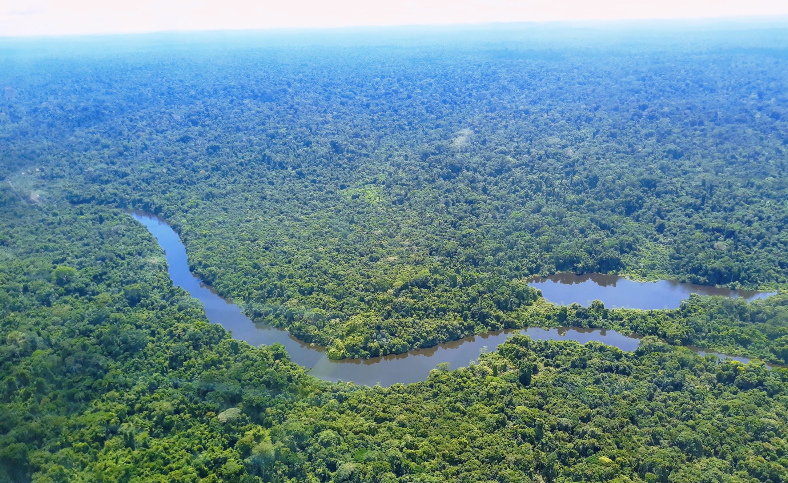
In training, the biggest bottleneck is rarely GPU memory or model size. It is a small number of field samples accessible across a vast, expensive, and logistically complex environment. This article grew out of repeated discussions and practical experiences with data in the Amazon rainforest. There, the problem manifests itself in its most vivid form. That means dense forests, difficult access, and a budget out of proportion to the landscape.
Our goal here is to discuss how to build geospatial machine learning models when collecting more field data is too expensive, too time-consuming, or simply not feasible. And “expensive” here is indescribable. A single forest inventory plot in a remote location can cost as much as a modern computer for training an ML model. The focus is not on ready-made recipes, but on practical trade-offs: what to simplify, where to normalize, how to validate, and how to communicate uncertainty when the dataset is much smaller than desired.
This problem occurs frequently in environmental, forestry, and remote sensing applications, but is not unique to these fields. This logic applies to continuous spatial variables where images, mosaics, and data cubes are abundant, but field labels are expensive, rare, and incomplete.
Structural challenges of geospatial data
Collecting data in the environmental field is always expensive. It requires planning, logistics, equipment, staff, and often a narrow seasonal window. In remote areas like the Amazon rainforest, access requires boats, long distance travel, and complex permits, significantly increasing costs. All of this makes each additional sample very expensive, and this also applies to tropical forests, arid regions, mountaintops, and oceans. While satellite pixels and spectral derivatives are relatively easy to obtain, reliable field measurements are logistically complex.
The typical scenario is familiar to anyone who works with environmental data. That is, a vast region of interest, a large collection of images, indexes, terrain models, and other remote sensing products, and a limited number of reference points or plots collected over different campaigns, sometimes even years apart.
At first glance, 100 to 200 samples may seem like a reasonable number to build a useful model. The problem is that raw sample size rarely tells the whole story in geospatial research. What may seem like a relatively comfortable data set overall can prove to be quite challenging once the heterogeneity of the environment begins to be explored.
Step 1 – Extract more information from each sample
When labels are missing, jumping directly to the most sophisticated model available is rarely the most productive method. The greatest benefits typically come from increasing the information content of each sample through data integration and feature engineering.
In practice, this means trying to represent each reference point with a small but informative set of complementary signals. Rather than relying on a single source of information, it is worth combining metrics from optical sensors, structural information from LiDAR and radar, topographic variables from DEMs, and temporal context when seasonal variations are important, such as floods and droughts in the Amazon.
The goal is not to use everything available to inflate the feature matrix. When you have less data, the chance that your model will learn incorrect relationships almost always increases. The goal is to condense the different physical dimensions of the landscape into a lean set of useful variables.
Step 2 – Choose a model that takes into account the actual size of the problem
When datasets are small, model selection is less about “who will beat the benchmark” and more about distributed control. Flexible models may seem appealing, but with so few labeled examples, the risk of memorizing local noise or accidental spatial patterns increases rapidly.
This often leaves tree-based algorithms as a strong equilibrium. Random forests as a robust baseline, gradient boosting such as XGBoost when more control and flexibility is needed, and more complex ensembles are only used when there is real evidence of stable gains. Their advantage is not magic, but a reasonable ability to handle nonlinearity, interactions, and moderate multicollinearity while providing a clear regularization mechanism.
In this context, some trade-offs always emerge. That is, a deeper model captures more details but remembers more noise. More features improve descriptive power, but increase the risk of overfitting. When data is small, the goal is not to maximize performance with one favorable split, but to find a configuration that is stable enough to remain meaningful even when the model moves beyond the neighborhood of the sampled points.
Step 3 – Verify without lying
The easiest way to fool yourself in geospatial machine learning is to apply random cross-validation to your spatial autocorrelation problem. Splitting adjacent samples between training and testing tends to artificially inflate metrics when nearby points share environment, history, and sensor artifacts.
This is the kind of mistake that produces great validation metrics in the lab, but produces completely distorted maps in real life. On paper, this model appears to be generalizing. In reality, you’re just interpolating within a neighborhood that’s already very similar to what you saw during training.

Spatial validation is therefore essential. The exact format may vary, but the logic is simple. Blocks that are spatially close should stay together so that the test set truly represents regions that the model does not see indirectly. This change will almost always degrade metrics compared to random verification, but its apparent setback is actually an increase in honesty.
Step 4 – Hidden class imbalance problem
Even after implementing spatial validation, there are still details that are often overlooked. An initial sample size of 100-200 seems to be sufficient as long as the study area is treated as homogeneous.
But when environmental analysis becomes more careful, another layer of complexity emerges. That is, the landscape does not function as a single system. In reality, a region is composed of different environmental layers or plant physiological structures, each with its own structural, mechanical, and spatial characteristics.

This completely changes the way you interpret sample size. That amount of data no longer represents a single problem. It is distributed in multiple ecological regions with different behaviors. The model is not learning from hundreds of equivalent examples, but from a smaller, unbalanced, and highly heterogeneous subset.
This is where the sense of methodological safety dissolves. Some layers end up being well represented, while others sit on the edge of minimally reliable in training and validation. Aggregated average performance may still appear acceptable, but uncertainty increases where sample coverage is weakest or where ecological behavior is most distinct. Focusing on average metrics is misleading. In heterogeneous scenarios, a good global average does not guarantee stable behavior across all parts of the map.
Step 5 – Treat uncertainty as a key product (and communicate limits)
When spatial heterogeneity fragments the effective sample size, uncertainty ceases to be a methodological footnote and becomes a central part of the artifact. Pretending there is uniform accuracy omits the real variation in error across space.
Uncertainty maps must therefore be treated as a core product rather than an optional appendix. This is a way to show where the model is supported by sufficient evidence and where it is extrapolating beyond what the data can sustain. Depending on the pipeline, this uncertainty can be approximated by tree-to-tree variation, validation-fold variance, or spatial analysis of out-of-fold residuals.
Users should not receive only a continuous surface of predicted values. A more responsible approach is to be transparent and make it clear that:
- The model was validated in a spatially consistent manner
- Different environment layers indicate different error levels
- Sample coverage directly impacts local reliability
- Uncertainty is part of the product, not a footnote

This attitude strengthens technical interpretation and prevents the misuse of maps that appear accurate but have uneven reliability.
If it is not possible to collect more data
The recommendation to “collect more data” is methodologically sound but operationally useless in many situations. In remote locations, cost, time, and logistics impose far more restrictive constraints than any modeling guideline is willing to admit.
This is precisely why geospatial problems require realism. If expanding the dataset is not practical, the alternative is to better leverage what exists. Test honestly, reduce complexity where necessary, extract more from covariates, and clearly communicate uncertainty. Small-scale data in geospatial work is not just a matter of quantity. It is a challenge to simultaneously address quantity, heterogeneity, and spatial distribution.
lessons learned
- sample size is an illusion: What matters is the effective sample size within each actual hierarchy or subenvironment of the problem.
- Spatial validation is non-negotiable: Random validation masks overfitting by ignoring spatial autocorrelation.
- Feature engineering overcomes complexity: Intelligent sensor integration goes beyond complex architectures with small datasets
- Using the Uncertainty Guide Map: Should be delivered along with the forecast to flag areas of extrapolation and sampling gaps.
Without data growth, the only honest path forward is to make uncertainty visible and make it part of the answer, not an excuse.


