Appendix: Evaluation of longitudinal models
To assess whether longitudinal features (1-month change variables) significantly improved model performance within this framework, we applied the same preprocessing, training, and evaluation pipeline to a combined feature set of 22 variables (11 baseline + 11 change features). The full longitudinal performance is reported in Table 2 along with the baseline results.
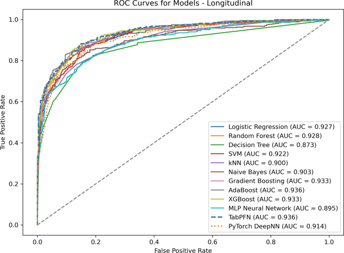
Across all 12 models, longitudinal AUC values ranged from 0.873 to 0.936, dominated by the ensemble method (TabPFN: 0.936, AdaBoost: 0.936, XGBoost: 0.933, Gradient Boosting: 0.933). Performance differences between the main models were minimal (\(\delta\)AUC < 0.003), consistent with the convergence pattern observed in the baseline model.
See Figure 7.

ROC curve of machine learning model using longitudinal features. Color-coded curves are computed on the retained test set. Diagonal dashed lines represent random classification. AUC values for each model are reported in the legend.
The top three models (TabPFN, XGBoost, and Gradient Boosting) were further evaluated using calibration analysis, threshold optimization, functional stability, and error profiling (Table 5). All models are well calibrated and have overlapping AUC confidence intervals (TabPFN: 0.922 to 0.950, XGBoost: 0.918 to 0.948, Gradient Boosting: 0.917 to 0.947). TabPFN has the lowest Brier score (0.0975) and the highest functional stability (\(\rho\) = 0.889), but had the highest number of false positives (n = 85). XGBoost achieved the best balance between false positives (n = 69) and false negatives (n = 68) and was selected as the final model based on favorable tradeoffs between performance, calibration, computational efficiency, and overall model properties.
SHAP analysis of the longitudinal XGBoost model confirmed that the importance ranking of core features was consistent with the baseline model, with perceived stress, RHR, sleep duration, and HRV remaining key predictors (Figure 8). Change-based features (e.g., HRV change, sleep efficiency change) provided additional interpretive value by capturing the direction of recovery trajectory, but did not supersede baseline features. This indicates that longitudinal features primarily refine interpretation and improve sensitivity to temporal variation, rather than fundamentally changing the relationship between learned features and outcomes.

SHAP-based interpretation of XGBoost models trained on longitudinal features. (be) Beeswarm plot summarizing the significance and direction of global features across all samples. (b) Dependency plot of perceived stress (0-10) versus SHAP value. Color indicates sleep time. (c) Dependence plot of RHR (bpm) versus SHAP value. Color indicates sleep time. (d) Waterfall plot showing the contribution of feature levels to individual predictions.


