An explainable AI framework for enhanced software defect prediction using transformer-assisted boosting

This section describes the approach for building and assessing the proposed TABF for software defect prediction. It outlines the datasets used, data pre-processing, the model design, and the evaluation metrics, aiming for accuracy, clarity, and prediction precision.

Data preparation and preprocessing

The data preparation phase concerns the cooperation with two publicly available datasets: the NASA Metrics Data Program (MDP)²⁶ and the Code4Code datasets²⁷. The experiments were based on these datasets. The NASA MDPs data is divided into sub-data, such as CM1, PC1, KC2, KC3, and MC1, each of which is further divided by programming paradigms, such as procedural (C) and object-oriented (C +  + , Java). These data include line counts (LOC) and measures of cyclomatic complexity and McCabe complexity, coupling and cohesion, Halstead measures, and maintainability index. For example, CM1 has 327 modules, and PC1 has 705 modules, and the percentages of defective modules vary (9.7 in CM1 and 6.9 in PC1). The Code4Code dataset is a complement to the NASA MDP, containing metrics for defect-prone software modules. It includes one line of code, the number of comments, Halstead measures (volume, difficulty, effort), the maintainability index, and the frequency of commits. These characteristics indicate the inherent and sustainable character of the software systems. The MDP and Code4Code datasets were selected because they are widely used benchmarks in software defect prediction, provide standardized static code metrics, and enable fair and reproducible comparison with prior studies across both traditional and modern software projects.

Table 1 provides a comparative overview of the NASA MDP and Code4Code datasets, highlighting differences in dataset size, feature composition, label definition, and defect prevalence to support reproducibility and fair evaluation.

Data cleaning

The data cleaning is a very important part of the pre-processing phase to make the data reliable and use it to train and test predictive models. It is here that the missing values, outliers, and standardizing scales are processed in such a way that the data is maintained intact and unaltered. The dataset of NASA MDP and Code4Code has class imbalances with defective modules constituting a minority group. To address this, the Synthetic Minority Over-sampling Technique (SMOTE) was applied to the training data to balance class distributions and reduce bias toward the majority class. Numerical features \({x}_{i}\in X\) with missing values were filled by applying a multivariate iterative imputation approach as opposed to simple mean or median imputation. This method approximates missing features as a regression equation of other related features using chained regression models. An example is that in predicting missing values of one another, Lines of Code, Halstead Volume, and McCabe Complexity metrics are used, thus maintaining relationships between features. Mathematically, the imputed value \({\widehat{x}}_{i}\) is estimated as:

where \(f\left(\cdot \right)\) represents an iteratively trained regression model with respect to all possible features \({X}_{-i}\) except \({x}_{i}\), and \(\theta\) represents learned parameters of the regression function.

Outlier detection was performed using the z-score method, defined as:

where \(\mu (X)\) and \(\sigma (X)\) are the mean and standard deviation of feature \(X\), respectively. Instances with \(\mid {z}_{i}\mid >3\) were treated as outliers and removed to reduce noise and skewness in the training data.

After imputation and outlier removal, Min–Max normalization was applied to scale all features into a comparable range \([\text{0,1}]\), as given by:

This transformation makes features contribute equally when training the model and stabilizes optimization by gradient.

Finally, one-hot encoding was used to operationalize categorical variables, where each category was assigned a unique binary number. Scaling was performed on numerical attributes to give the features an even distribution. The large data-cleaning pipeline, consisting of repeated imputation, outlier detection, normalization, and encoding, ensured reduced bias, fewer abnormalities, and a high-quality and standardized dataset that may be subsequently reused in further feature engineering and model building.

Feature engineering (domain-specific knowledge)

Software defect prediction is based on feature engineering, where data and domain knowledge are combined to produce significant features out of raw datasets. The features generated based on the NASA MDP and Code4Code datasets are based on the high-level software engineering principles to extract features that indicate defect proneness.

We extract features such as lines of code (LOC), cyclomatic complexity, McCabe’s complexity, object-oriented metrics, coupling, and cohesion from the NASA MDP dataset. These features quantify the structural and logical quantities of the code. Similarly, the Code4Code dataset includes attributes like volume, difficulty, effort (Halstead metrics), maintainability index, number of defects, and commit frequency to reveal coding patterns and development activity. The NASA MDP and Code4Code repositories have slight differences in the number of features and names assigned to features, but to guarantee compatibility and fairness in cross-dataset analysis, the features that were shared across the two datasets were utilized. The measures that have been retained are Lines of Code (LOC), McCabe Cyclomatic Complexity (CC), Halstead Volume (HV), Halstead Effort (HE), Comment Density (CD) and Module Size (MS). All these features were normalized and standardized before they were trained to maintain constant semantics and scale across datasets.

Table 2 shows the features engineered from both datasets, grouping them into basic metrics, cyclomatic complexity metrics, object-oriented metrics, Halstead metrics, and other relevant attributes. However, this domain-driven approach guarantees that the features are interpretable and aligned with traditional software quality and defect prediction paradigms.

Model architecture

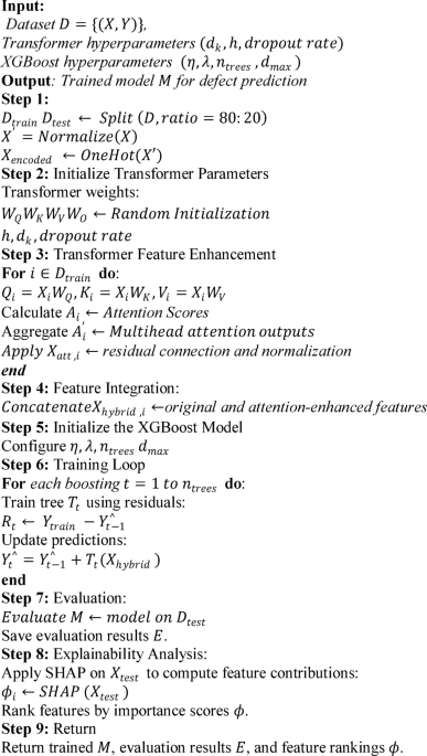
The proposed TABF architecture uses gradient boosting and attention mechanisms to improve software defect prediction. This hybrid approach combines the high efficiency of XGBoost with the interpretive power of transformer-based attention and is specifically adapted to the challenges of NASA MDP and Code4Code datasets. Algorithm 1 presents the TABF training.

Transformer-based feature learning and the XGBoost classifier are the biggest sources of time complexity of Algorithm 1. A complexity of \(O(n\cdot {d}^{2})\) is incurred by the Transformer, where nis the number of instances and \(d\) the number of features, whereas XGBoost takes about \(O(T\cdot n\text{log}n)\) for \(T\) trees. This complexity is \(O({d}^{2}+T\cdot d)\) in total space, including attention weights and tree structures. In TABF, the Transformer is used to transform features by producing a d-dimensional embedding for each software module; that is, it maps features with relationships within the context of the input metrics rather than simply reweighting features with a scalar metric.

XGBoost as base model

The architecture is based on the Extreme Gradient Boosting (XGBoost) algorithm, a powerful machine learning method known for handling structured data and achieving state-of-the-art performance on classification tasks. XGBoost is built on decision tree ensembles, leveraging gradient-boosting to minimize loss functions and iteratively improve predictive performance. Mathematically, the output of the XGBoost model is expressed as:

where \({\widehat{y}}_{i}\) is the predicted value, for instance \(i\), \(K\) represents the total number of trees, ​ \({f}_{k}\) are decision trees from the functional space \(F\), and \({x}_{i}\) denotes the input features. Each tree \({f}_{k}\)​ is trained to optimize the loss function \(L\), defined as:

where \(l\left({y}_{i},{\widehat{y}}_{i}\right)\) represents the primary loss (e.g., log loss for classification), and \(\Omega ({f}_{k})\) is a regularization term to prevent overfitting. XGBoost’s capability to process tabular data efficiently makes it an ideal base for structured datasets like NASA MDP and Code4Code, which contain numerical and categorical features crucial for defect prediction.

Attention mechanism (applied at the feature level)

The feature level uses attention mechanisms, which have become quite common in natural language processing, to highlight the most essential traits of defect prediction. This is how the model assigns weights to different features: those with higher predictive value receive higher weights. In every input instance, \({x}_{i}=[{x}_{i1}, {x}_{i2},{x}_{i3}\dots .,{x}_{id}]\), the attention mechanism will calculate the weighted representation \({z}_{i}\) as:

where \({\alpha }_{j}\) denotes the attention weight for the \({j}^{th}\) feature and satisfies the following constraints:

These weights are learnt during the training process, such that those features which influence the prediction of defects more effectively will receive a higher weight. In the final stages of fine-tuning, the feature importance scores obtained by SHAP were scaled to feature-level attention weights of the Transformer, which were then biased by the empirically significant metrics, but could still be further optimized by the backpropagation process.

Hybrid XGBoost-transformer model

The hybrid model combines both XGBoost and Transformer-based attention mechanism to merge their capabilities in defect prediction. The architecture runs in a pipeline manner. Input features are first handled by Transformer encoder which computes weights of attention in order to highlight the most important features producing a weighted feature vector. This weighted vector is subsequently sent to XGBoost that goes through feature splitting and decision tree based transformations. Lastly, XGBoost sums up the decision trees to come up with the final defect prediction.

The attention weights in the Transformer encoder are computed by a scaled dot-product mechanism, which is as follows:

The matrices of query, key and value, \(Q\), \(K\), and \(V\), are obtained using the input features and d K is the dimensions of the keys. This works to ensure that the model is effective in detecting and ranking the most important features, to predict defects using complementary abilities of XGBoost and the attention mechanism of the Transformer as shown in Fig. 1.

Figure 1 illustrates the application of the Transformer encoder, which uses attention mechanisms to prioritize important features in creating weighted feature vectors. Processing these vectors involves the XGBoost classifier, which uses its ensemble learning feature to provide strong forecasts of bad and non-bad software modules. The choice of XGBoost as the downstream classifier in the Transformer-Assisted Boosting Framework (TABF) is not arbitrary or without theoretical justification. Although the Transformer encoder acquires global dependencies and dynamically reweights input metrics with self-attention, XGBoost is more effective at modeling nonlinear relationships on structured data through gradient-boosted decision trees. TABF has the advantage of learning contextual representations and efficient gradient-boosting optimization by feeding attention-enhanced feature embeddings into XGBoost. The combination of this integration supports the model to be generalized to heterogeneous software metrics and explain them with features attributed via SHAP.

Loss functions

The loss function directs the training of a model and compares how far the estimated label and actual label are. In the case of software defect prediction, the hybrid XGBoost-Transformer model is applied, which is based on loss functions that are related to the classification task and optimization requirements of the sub-elements of the model. In the case of the XGBoost part, binary cross-entropy as the main loss function is applied to solve the binary classification problem. Given a collection of N samples, the binary cross-entropy loss is given as:

where \({y}_{i}\in \{\text{0,1}\}\) is the true label, and \({\widehat{y}}_{i}\) is the predicted probability of the positive class. This loss penalizes incorrect predictions based on confidence, ensuring the model assigns higher probabilities to true labels. The XGBoost component incorporates a regularization term into the loss function to prevent overfitting. The complete loss is:

where \(Reg(\Theta )\) defined as a penalty on the model parameters Theta (i.e. weight regularization as L2 norm), and the regularization strength is determined by λ. This will make the model applicable to unknown data. The attention mechanism of the Transformer encoder is defined to minimize the same binary cross-entropy loss. Still, the attention weights are also tuned to balance the attention, giving more weight to features with high predictive importance. Backpropagation is implicitly performed through attention weights, which are trainable parameters that update during gradient descent.

The optimization algorithm will ensure that the hybrid model minimizes its loss function during training. The Transformer encoder and the XGBoost classifier are optimized differently, but complementary to each other. The attention mechanism in the Transformer encoder is learnt with stochastic gradient descent (SGD) or its variants, such as Adam. The update rule of the parameter \({\Theta }_{t}\)​ at iteration \(t\) is:

where η is the learning rate, and \(\nabla_{\Theta } L\) is the gradient of the loss concerning \(\Theta_{t}\). Adam, a popular variant of SGD, uses adaptive learning rates and momentum to accelerate convergence:

where \({m}_{t}\) and \({v}_{t}\) are first- and second-moment estimates, \({\beta }_{1}\) and \({\beta }_{2}\) are decay rates, and \(\epsilon\) ensures numerical stability. XGBoost optimizes its decision trees using a second-order gradient boosting technique. At each step, the algorithm constructs a tree that minimizes the loss function by approximating the loss with its Taylor expansion:

Here \(g_{i} = \frac{\partial L}{{\partial y_{i}^{ \wedge } }}\) and \(h_{i} = \frac{{\partial^{2} L}}{{\partial y_{i}^{2 \wedge } }}\) are the loss’s first- and second-order gradients concerning the predictions. The regularization term \(\Omega \left( {f_{t} } \right)\) penalizes tree complexity to avoid overfitting. Combining these optimization strategies ensures that both components of the hybrid model converge efficiently to a solution that minimizes classification error while maintaining interpretability and robustness.

Model training and hyperparameter tuning

The study provides a complete framework of training and testing the TABF to be able to predict software defects. This is a step by step process that entails training, the adjustment of hyperparameters, and optimization.

TABF is trained in two major processes, that is, feature encoding and classification. In the first stage, the Transformer encoder is employed, and attention is calculated to create xenophrastic features with the highest importance. These feature weights are then fed into the XGBoost classifier, which uses decision tree ensembles as a predictor of defects. The training process is to minimize a loss function L, which is defined as:

where \(l{(y}_{i},{\widehat{y}}_{i})\) is the primary loss function (e.g., binary cross-entropy for classification), \(\lambda\) is a regularization parameter, and \(Reg(\Theta )\) penalizes complex models to prevent overfitting.

Two strategies for optimization of the model are employed. Firstly, In the Transformer encoder, the attention weights are learned through gradient descent by backpropagating errors so that relevant features are given more attention. The optimization process follows:

where \({\Theta }_{t}\) represents the model parameters at iteration \(t\), \(\eta\) is the learning rate and \({\nabla }_{\Theta }L\) is the gradient of the loss concerning \(\Theta\).

Second, the XGBoost component optimizes decision trees using second-order gradient boosting. At each step, the objective function is expanded into a Taylor series as:

where \({g}_{i}\) and \({h}_{i}\) are respectively first and second order gradients of the loss concerning the predictions and \(\Omega \left({f}_{t}\right)\) is a regularization term for tree complexity. Transformer-Assisted Boosting Framework balances accuracy and generalization by iteratively optimizing the attention mechanism and the decision trees to relieve the earlier overfitting and underfitting problems. Reliable and interpretable predictions are ensured through this complete training and evaluation process.

The TABF’s performance hinges on careful hyperparameter tuning, and we make use of grid search with cross-validation to maximize accuracy. We tune the number of attention heads \((H)\), embedding size \({d}_{model}\), and dropout rate \((p)\) for the Transformer encoder to improve feature representation and reduce overfitting. For the XGBoost classifier, we fine tune the parameters of the learning rate \((\eta )\), maximum tree depth \((d)\), number of estimators \((K)\), and regularization parameters \((\lambda ,\alpha )\) to reach a balance between complexity, and generalization. k-fold cross-validation is a technique to provide high reliability for a hypothesis evaluated in a grid search over predefined parameter ranges. This systematic approach gives the TABF optimal performance and robust generalization.

Experimental setup and evaluation metrics

All experiments were conducted using a consistent and reproducible evaluation protocol. The proposed TABF model and baseline methods were implemented in Python using PyTorch for the Transformer component, XGBoost for classification, and scikit-learn and SHAP for evaluation and explainability. Model training and evaluation were performed under the same preprocessing and data splitting settings to ensure fair comparison across methods. The experiments were executed on a workstation equipped with an Intel Core i7 processor, 32 GB RAM, and an NVIDIA GTX 1080 GPU, with CUDA used to accelerate training where applicable.

The performance of software defect prediction when utilizing the TABF is measured using evaluation metrics. Several such measures are broadly used to assess a classifier’s performance, including accuracy, precision, recall meter, and F1 score, which can handle the issue of imbalanced data. Advanced measures such as AUC-ROC and log losses provide extra information about probabilistic estimates and the model’s discriminant capabilities, making for an integrated and uniform evaluation of the model. In benchmarking, we used Random Forest, SVM, and LSTM which are ensemble-based paradigm, kernel-based paradigm and deep sequence-learning paradigm respectively. This triad was selected to have a balanced comparison between traditional machine learning and deep learning categories, which are also in line with the previous software-defect prediction research.