
Study design and participants
The Gulf Long-term Follow-up (GuLF) Study, as previously described [24], is a prospective cohort study designed to examine human health effects following the 2010 Deepwater Horizon (DWH) oil spill in the Gulf of Mexico. A total of 32,608 adults (≥21 years old) participated in the GuLF Study. Participants completed a 30- to 60-min computer-assisted telephone enrollment interview, and English and Spanish-speaking participants from eastern Texas, Louisiana, Mississippi, Alabama, and Florida (n = 26,828) were invited to complete a home visit. Between May 2011 and May 2013, 11, 193 participants completed the home visit, which included biological sample collection, functional measures (e.g., blood pressure, lung function), anthropometric measurements, and examiner-administered questionnaires. Of those, we included data from 11,071 participants in our analysis. After excluding participants with unknown race or ethnicity, missing geocodes and environmental predictors of interest, 10,491 participants were included in the final analysis (Supplementary Fig. SA1 Sample Size Flowchart). The GuLF Study home visit data were collected using standardized protocols with training and quality control procedures as described previously [24]. Home visit participants provided written informed consent. The study was approved by the Institutional Review Board of the National Institutes of Health.
Outcome ascertainment
Hypertension status was determined based on blood pressure measurements and antihypertensive medication use. Blood pressure was measured three times during the home visit following a standardized protocol, and the average of the last two measurements was used. Medication use was assessed via self-reported questionnaires and confirmed by examiner visualization of medications. Participants were defined as having hypertension if they met any of the following criteria: 1) systolic blood pressure ≥140 mmHg; 2) diastolic blood pressure ≥90 mmHg; or 3) current use of any antihypertensive medications [25].
Predictor variables and environmental exposure data
Demographic and anthropometric predictors
The base model (details described in the Statistical Analysis section) included age, sex, race/ethnicity (non-Hispanic White, non-Hispanic Black, Asian, Hispanic, and other), and measured BMI (body mass index, continuous), as these predictors are well-established hypertension risk factors and commonly available in large epidemiological datasets. These characteristics were collected via the enrollment questionnaire and during the home visit.
Environmental exposure predictors
Environmental predictors were selected based on previously established associations with hypertension or hypotheses informed by domain expertise in environmental epidemiology, supported by prior peer-reviewed studies. Data availability was also a determining factor, with sources including publicly accessible datasets and geospatial datasets previously linked to cohorts led by the Epidemiology Branch of the National Institute of Environmental Health Sciences (NIEHS).
All environmental predictors were linked to participants’ geocoded home visit addresses using the spatial unit provided by each dataset (for example, census tract or block group, or 1 km by 1 km grid). The spatial resolution and exposure time window for each predictor are summarized in Supplementary Table A1. Predictors representing longer-term neighborhood context (for example, neighborhood social indices and land cover) were assigned based on the dataset year available for that measure. Ambient exposures (for example, air pollution and temperature metrics) were derived using prespecified windows anchored to the home visit date when daily or gridded data were available (for example, annual mean in the 365 days prior to the visit). For predictors only available as a single calendar-year estimate, we assigned that year’s value to all participants.
Environmental predictors were categorized into two major categories: (1) Neighborhood social environmental predictors and (2) Ambient environmental predictors. Occupational and residential oil spill-related exposure measures were also considered. Details about spatial resolution, time window, and data sources are provided in Supplementary Table A1.
Neighborhood social environmental predictors
Neighborhood predictors were linked at the census tract or block group level, including the Area Deprivation Index (ADI), Social Vulnerability Index (SOVI), and Community Resilience Scores (CRS).
The ADI (2013, percentile, census block group level) is a ranked composite measure of neighborhood disadvantage based on education, employment, housing quality, and poverty indicators derived from the U.S. Census and the American Community Survey. Higher values indicate greater neighborhood disadvantage [26].
The SOVI (2010, percentile, census tract level) was developed by the Agency for Toxic Substances and Disease Registry and the Centers for Disease Control and Prevention. This index quantifies the susceptibility of social groups to adverse impacts from natural hazards, including disproportionate death, injury, loss, or disruption of livelihood. Higher values indicate greater vulnerability [27].
The CRS (2010, index, census tract level) measures a community’s ability to prepare for anticipated natural hazards, adapt to changing conditions, and recover rapidly from disruptions. This measure is provided by the Hazards Vulnerability & Resilience Institute at the University of South Carolina. Higher values indicate greater resilience [28].
Ambient environmental predictors
Ambient environmental exposures included air pollutants, air toxics, extreme temperature measures, and nighttime light, linked at the census tract or grid level.
Fine particulate matter (PM₂.₅) and nitrogen dioxide (NO₂) (average over 365 days prior to a home visit, 1 km × 1 km grid level) were obtained from National Aeronautics and Space Administration’s (NASA) Socioeconomic Data and Applications Center (SEDAC) [29, 30]. Exposures were calculated as the annual average concentration over the 365 days preceding each participant’s home visit.
The national air toxics assessment (NATA) (2011, census tract level) dataset from the U.S. Environmental Protection Agency (EPA) estimated calendar year average ambient exposure to multiple hazardous air pollutants [31]. Based on prior studies linking air toxics to hypertension, we included: acetaldehyde, acrolein, antimony, arsenic, benzene, biphenyl, butadiene, cadmium, chromium, cobalt, diesel, formaldehyde, lead, manganese, mercury, naphthalene, polycyclic organic matter, selenium, and styrene [32].
The WetBulb globe temperature (WBGT) (average over 7-day, 14-day, 30-day, and 365-day periods prior to the home visit, 1 km × 1 km grid level) was obtained from NASA Daymet [33]. WBGT measures heat stress in direct sunlight, accounting for temperature, humidity, wind speed, and solar radiation using Bernard and Iheanacho’s approximation [27]. The number of extreme heat days was also calculated as the total number of days in the 365 days preceding home visit where WBGT exceeded 25 °C, serving as a long-term heat exposure indicator.
Nighttime light exposure (calendar annual average for the 365 days prior to home visit completion, 1 km × 1 km grid level) was obtained from a harmonized dataset integrating measurements from the Defense Meteorological Satellite Program and the Visible Infrared Imaging Radiometer Suite. Higher values indicate greater artificial light exposure [34].
Elevation, land cover, and vegetation were included to represent environmental and geographic characteristics linked at 1 km × 1 km grid level.
Elevation (2011 or home visit, 1 km × 1 km grid level) was obtained from WorldClim, reflecting terrain characteristics [35].
Land cover (2011, 1 km × 1 km grid level) was derived from the National Land Cover Database. The most frequent land cover types (e.g., developed space, forest, agriculture, and others) within each grid were assigned to participants to represent their surrounding environment, based on data from the Multi-Resolution Land Characteristics Consortium [36].
The normalized difference vegetation index (NDVI) (2011–2013 monthly average, 1 km × 1 km grid level) is a satellite-derived measure of green space, obtained from NASA Moderate Resolution Imaging Spectroradiometer (MODIS) [37]. A single NDVI value at each participant’s residential address was calculated as the average of all monthly values from 2011 to 2013. Higher values indicate greater vegetation density.
The National Risk Index (NRI) (2020, census tract level) estimates expected annual losses from natural hazards across the U.S. based on experiences over the past twenty years Given the study’s location in the Gulf coast region, we included indices for drought, heat wave, hurricane, riverine flooding, strong wind, and tornado [38].
Hurricane Katrina and Hurricane Isaac Exposure (self-reported at home visit, individual level) was assessed through questionnaires in which participants reported whether they experienced financial losses, relocation, or health consequences due to these hurricanes (Yes/No).
Oil-spill-related predictors
Given the study population of DWH oil spill cleanup workers, occupational and residential level oil-spill-related exposure measures were included in a secondary analysis.
The Oil-Spill Cleanup Worker Status (ever worked at least one day on oil-spill clean-up, individual level) classified participants as ever or never having participated in oil spill response and cleanup efforts (yes/no).
Residential proximity to the Gulf Coast (home visit, county/parish level) was determined based on whether participants resided in a county or parish abutting the Gulf of Mexico or further from the coast (direct contact/indirect contact/other Gulf state residence). This measure served as a broad geographic proxy for potential environmental exposure related to the oil spill and coastal ecosystem changes.
Total hydrocarbon concentration (maximum daily exposure during cleanup measured as ppm days, individual level) was estimated using a job-exposure matrix that integrated field measurements of airborne contaminants (>28,000 full-shift personal air samples taken with passive organic vapor dosimeters at the time of oil spill response and cleanup efforts) for specific cleanup tasks with self-reported job histories.
Statistical analysis
The dataset split into a training set (70%) and a testing set (30%) using weighted random sampling to achieve the same hypertension prevalence across both sets. All model development, including variable selection and model training, was conducted using the training set, and model performance was evaluated on the test set. During preprocessing, missing values, as outlined in Supplementary Fig. SA1, were excluded. Dummy variables were created for categorical variables (race/ethnicity, land cover, and proximity to Gulf coast). Continuous variables were normalized within the training and test sets separately to avoid information leakage.
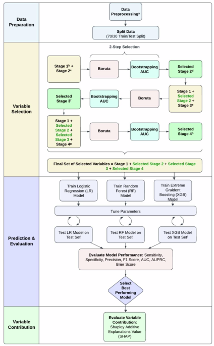
To assess the incremental predictive value of environmental predictors, we implemented a staged modeling pipeline, as illustrated in Fig. 1. The base model (Stage 1) included age, sex, race, and BMI, well-established hypertension risk factors, retained across all subsequent stages. In Stage 2, neighborhood social environmental variables were added to Stage 1. Stage 3 added ambient environmental variables to Stage 2 (i.e., Stage 2 + ambient exposures). Oil-spill-related variables, unique to this cohort, were introduced in a fourth stage (Stage 4) as a secondary analysis, with results shown in Supplementary Table A2. A sensitivity analysis was also conducted in which the introduction order of the variables was reversed, such that ambient environmental variables were added in Stage 2 and neighborhood environmental variables were added in Stage 3. The results for this sensitivity analyses are shown in Supplementary Table A5.

a Data preprocessing steps included addressing missing values, creating dummy variables for categorical variables, and standardizing data after splitting. b Stage 1 variables: Age, Sex, Race/Ethnicity, BMI. c Pre-selection Stage 2 variables: Social vulnerability index, Area Deprivation Index, Community Resilience Score. d Selected stage 2 variables: Social vulnerability index, Area Deprivation Index, Community Resilience Score. e Pre-selection Stage 3 variables: PM2.5, NO2, acetaldehyde, acrolein, antimony, arsenic, benzene, biphenyl, butadiene, cadmium, chromium, cobalt, diesel, formaldehyde, lead, manganese, mercury, naphthalene, polycyclic aromatic hydrocarbons, selenium, styrene, WetBulb globe temperature (7 day, 14, day, 30 day, 365 day), nighttime light, elevation, landcover, vegetation index, drought risk index, heat wave index, hurricane risk index, riverine flooding risk index, strong wind risk index, tornado risk index, hurricane Katrina impact, and hurricane Isaac impact. f Selected stage 3 variables: PM2.5, vegetation index, Formaldehyde, and NO2. g Pre-Selection Stage 4 variables: Total hydrocarbon exposure, residential proximity to oil spill, oil spill cleanup worker status. h Selected stage 4 variables: Total hydrocarbon exposure. i Variables were added to the model and evaluated in stages: Stage 1 (stage 1), Stage 2 (stage 1+ selected stage 2), Stage 3 (stage 1+ selected stage 2+ selected stage 3), Stage 3 (stage 1+ selected stage 2+ selected stage 3+ selected Stage 4). Performance metrics were recorded and compared for each stage and model.
Variable selection was performed within exposure domains to maintain stage interpretability: neighborhood social candidates were screened for Stage 2; ambient candidates were screened for Stage 3 conditional on retaining Stage 2 variables. We used a two-step procedure. First, the Boruta algorithm identified relevant predictors by comparing their importance scores to those of randomly permuted “shadow” variables; variables with significantly higher importance were retained [39]. Second, a bootstrapped leave-one-out approach was used to assess each variable’s contribution to prediction. Specifically, the training set was resampled 1000 times with replacement. For each bootstrap, a selected variable was removed from the model, and the resulting change in area under the precision-recall curve (AUPRC) was recorded. Variables were retained if their exclusion resulted in a significantly greater-than-expected frequency of AUPRC decreases, as determined by a one-sided binomial test. Further details on the Boruta algorithm and AUPRC bootstrapping procedure are provided in the Supplemental Methods.
We trained Logistic Regression (LR), Random Forest (RF), and Extreme Gradient Boosting (XGB) models using the selected variables in the aforementioned stages. Hyperparameters were optimized using Optuna [40], and the model with the best overall performance was selected for interpretation. Model performance was assessed on the test set using area under the receiver operating characteristic curve (AUC), area under the precision-recall curve (AUPRC), Brier score, sensitivity (recall), specificity, precision, and F1 score. The Brier score assessed the calibration of predicted probabilities, with lower values indicating better alignment between predicted and observed outcomes. The F1 score, the harmonic mean of precision and recall, reflects the balance between false positives and false negatives.
AUC, AUPRC, and Brier score are threshold-independent metrics that evaluate overall model performance without relying on a specific classification cutoff, reflecting discrimination, calibration, and performance across all possible thresholds. In contrast, threshold-specific performance metrics (sensitivity, specificity, precision, and F1 score) were computed at multiple probability cutoffs and are reported in Supplementary Table A3.
To interpret variable contributions, we applied Shapley Additive exPlanations (SHAP) [41] to the final model. SHAP assigns importance values to each feature based on its contribution to individual-level predictions, indicating whether the feature increases or decreases predicted hypertension risk.
We conducted stratified analyses by age group (<50 vs. ≥50 years) and sex to assess potential variation in model performance. All analyses were performed using Python 3.6.8.

