Machine learning applications for predicting safety incidents in construction industry

Data collection

The research study outlined in this paper comprised two primary segments. The initial phase focused on constructing a database of construction accidents for statistical analysis. This involved the collection of reports from an initial dataset of 250 construction accidents resulting in either fatal or nonfatal injuries. However, 47 incidents were excluded due to missing or incomplete data in critical explanatory variables, such as time with employer, time of incident, and specific PPE types. These exclusions were necessary to ensure data quality and reliability, leaving 203 incidents as the final dataset used for model development and analysis. The second phase of the study involved developing comprehensive ML models to predict the nature (NOI) and severity (SOI) of construction incidents, providing a useful framework for preventing future accidents.

For data collection, a structured questionnaire was developed and circulated (attached as Annex A). The dataset consists of construction-based safety incidents from Saudi Arabia, primarily from Makkah and Riyadh regions, covering incidents from 2018 to 2024.

The study categorizes safety incidents according to the Occupational Injury and Illness Classification System (OIICS)²².

1. 1.

   Nature of incident: The statement delineates the primary physiological attributes of the injury. Several prevalent types of fatalities in the construction industry encompass bruises, falls, burns, fractures, electrical shock, and traffic accidents.

2. 2.

   Severity level of incident: Numerical value representing the severity of the incident on a pre-defined scale of 1–5, where 1 is minor and 5 is fatal.

The OIICS²² offers comprehensive information regarding deaths, encompassing the physical attributes of the victims (such as the kind of the injury and the specific part of the body affected) as well as the origins and occurrences that lead to fatalities (including the cause of the injury and the incident or exposure). It is widely held that employing such a method, as opposed to relying just on a single dependent variable such as the risk of fatality, can yield more valuable insights and enhance the preparedness of pertinent stakeholders in comprehending and mitigating fatalities. Following a thorough analysis, data regarding each incident is gathered from the employer, coworkers present at the site, safety personnel, members of the onsite emergency response team, and other individuals who have witnessed the incident²². To minimize potential biases from subjective reporting, the collected data was cross validated using official injury logs maintained by site safety officers, ensuring consistency and accuracy in the reported details. Additionally, a standardized questionnaire was used during data collection to ensure uniformity in responses and reduce variability in subjective accounts. In cases of discrepancies between witness accounts and injury logs, priority was given to documented records to enhance data reliability. This study utilizes a set of input and output variables, which are presented in Table 2 with related numerical digit.

Data preprocessing

Data preparation involved the following steps. First, the categorical output variables (NOI and SOI) were compiled and restructured according to the questionnaire. Following an extensive examination of existing literature^16,19,23, a total of 17 explanatory factors were initially selected for predicting fatality severity. However, three variables, time with employer, fall height, and day/nighttime were excluded due to excessive missing data. The omission of fall height and day/nighttime is particularly noteworthy, as these factors could significantly influence incident severity. Fall height is directly correlated with injury severity in fall-related incidents, while day/nighttime conditions may impact visibility and worker fatigue, potentially increasing accident risks. Given their potential predictive value, imputation methods were explored to retain these variables. However, due to the high proportion of missing values, simple mean imputation risked introducing bias, and regression-based imputation did not yield reliable patterns due to data sparsity. Thus, these variables were excluded to maintain dataset integrity and avoid introducing artificial correlations. Future studies with more complete datasets could explore their predictive potential further. The remaining 14 variables have been retained for prediction. Additionally, NOI was incorporated as an explanatory feature to improve SOI prediction. Ultimately, any fatality data that contains missing figures is eliminated. Consequently, a comprehensive dataset of 203 fatalities has been established, encompassing 2 dependent variables and 14 explanatory variables.

Dataset overview and characteristics

To provide a clear understanding of the modelling dataset after encoding (Sect. “Encoding categorical data”), Table 3 presents the descriptive statistics of the 14 explanatory variables and the target (SOI). The table summarizes the mean, standard deviation, minimum, and maximum values, which help readers understand the distribution and scale of the encoded variables used in model training. These statistics establish the quantitative profile of the dataset and complement the categorical distributions illustrated in Fig. 1.

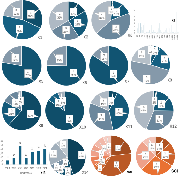
This analysis examines construction incidents reported between 2018 and 2024. Among the 203 incidents, the proportional distribution of severity levels, as defined by the SOI classification framework, is as follows:

• SOI Level 1 (Minor Incidents): 14%.

• SOI Level 2 (Moderate Incidents): 20%.

• SOI Level 3 (Severe but Non-Fatal Incidents): 29%.

• SOI Level 4 (Critical Incidents, Life-Threatening): 26%.

• SOI Level 5 (Fatal Incidents): 11%.

The distribution (Fig. 1) highlights that most incidents fall into moderate to severe categories (SOI Levels 2–4), while fatal incidents (SOI Level 5) represent a smaller yet critical portion of the dataset (11%). The most frequent injury type was mild, involving cuts, bruises, or fractures. Falls were the leading cause of these minor injuries, with scaffolding areas accounting for a significant portion (45%) as indicated by variable X14. Workshops were the second most common location for incidents (22% – X14), often involving multiple mishaps. Road areas followed at 10%, where traffic accidents were the primary cause of fatalities.

Examination of explanatory variables reveals concerning trends. A significant number of employers (25% – X6) failed to provide adequate safety training programs, and 16% (X7) neglected to enforce Personal Protective Equipment (PPE) use during construction. These gaps in employer practices, such as insufficient safety training and lack of PPE enforcement, may contribute to construction fatalities, as indicated by the reported deficiencies in these areas.

Handling imbalanced classes

The dataset exhibited a significant class imbalance, with fatalities (SOI Level 5) accounting for only 11% of the total incidents. Such imbalance can bias ML models toward majority classes, reducing their ability to predict minority outcomes like fatalities. To address this challenge, the Synthetic Minority Oversampling Technique (SMOTE)²⁴ was applied during preprocessing to generate synthetic samples for the minority class (SOI Level 5). This technique works by creating new data points in the feature space based on existing samples, ensuring that the minority class is sufficiently represented during model training. Moreover, for models such as XGB and GB, class weights were assigned inversely proportional to class frequencies. This adjustment penalized misclassifications of the minority class, ensuring that fatalities were prioritized without overfitting.

Dataset partitioning and feature scaling

The dataset utilized for the development of different models was divided into two distinct groups: a training set, employed for training the algorithms, and a testing set, utilized for evaluating the performance of the algorithms. The dataset was partitioned using an 80 − 20 training-testing split, following methodologies established in previous literature. Furthermore, to ensure proper feature scaling, we applied standardization (mean = 0, standard deviation = 1) selectively to models that are sensitive to feature scales, such as SVM and KNN. However, tree-based models, including RF, DT, and XGB, are inherently scale-invariant and do not require standardization. For these models, raw feature values were used without transformation to avoid unnecessary computations and potential biases. This procedure facilitates the standardization of all features, hence enhancing convergence throughout the training phase. In addition, one hot encoding technique is utilized to transform category information into numerical representations^25,26,27.

Encoding categorical data

To ensure compatibility with ML models, all categorical variables in the dataset, including NOI, PPE usage, incident location, weather conditions, and other explanatory factors, were transformed using Label Encoding. This method assigns a unique numerical value to each categorical class, allowing ML models to process the data efficiently without increasing dataset dimensionality.

Label Encoding was applied uniformly across both multi-class and binary categorical variables. For instance, in the case of NOI, each type of incident was assigned a numeric value (e.g., “Fall” = 0, “Collision” = 1, “Fire” = 2), ensuring that the variable could be effectively used in predictive modelling. Similarly, binary categorical features such as PPE usage (Yes/No) were also label-encoded (e.g., “No” = 0, “Yes” = 1), rather than employing one-hot encoding, which would have increased dataset complexity by creating multiple additional columns.

This approach was chosen because ML models like XGB, RF and DT inherently handle encoded numerical data, meaning that categorical features do not need additional transformation. By applying Label Encoding uniformly to all categorical data, the dataset was structured in a way that optimized both computational efficiency and predictive performance, ensuring that the models could effectively capture relationships between categorical variables and SOI.

Multicollinearity analysis

The importance of NOI in predicting SOI raises concerns about potential multicollinearity between NOI and other explanatory variables, therefore, a correlation analysis was conducted to assess relationships between explanatory variables. Figure 2 presents a correlation heatmap, illustrating the strength of associations among key features. The results indicate moderate correlations between NOI and PPE use, location, and precipitation, suggesting that while some dependencies exist, they are not strong enough to cause multicollinearity issues. The acceptable correlation threshold for avoiding multicollinearity concerns is typically below 0.70–0.80²⁸. In this study, all feature correlations remained below 0.85, ensuring that the model’s feature importance analysis remains valid and interpretable. Since ML models like XGB and RF are inherently robust to correlated features, multicollinearity does not significantly affect their predictions. Unlike regression models, where high multicollinearity (correlation > 0.85) can distort coefficient estimates, tree-based models can handle feature dependencies through internal feature selection and importance weighting. Therefore, no further adjustments (such as feature removal or dimensionality reduction) were required. These results confirm the independent contributions of key variables like NOI, precipitation, and PPE use in predicting SOI while ensuring that multicollinearity remains within acceptable limits.

Machine learning algorithms

For predicting such parameters, several ML models are employed to predict and classify such as K-Nearest Neighbours (KNN), Support Vector Machine (SVM), DT, RF, Gradient Boosting (GB) and Extreme Gradient Boosting (XGB). These models are conducted using the python language in Google Colab. The ML models, in conjunction with computational packages, have undergone significant advancements and have been successfully utilized in forecasting the safety incident features in the construction industry, as highlighted in prior studies^{19,23,29,30,31,32}.

The rationale for selecting these models lies in their proven strengths as described in Table 1. XGB and RF were chosen for their ability to handle non-linear relationships and feature interactions, which are critical in analysing the complex factors contributing to safety incidents. DT was included for its simplicity and interpretability, while SVM and KNN are well-suited for smaller datasets, aligning with the size of this study’s dataset. Deep learning models, such as artificial neural networks (ANN), were not employed due to their high risk of overfitting when applied to small datasets³³. The following sub sections describes about the models utilized in this study.

K nearest neighbour

In regression tasks, a non-parametric method called KNN regression can be useful. This approach forecasts the target value for a new data point by taking a mean of the output values of its K most similar neighbours within the training data. To determine how similar data points are, a distance metric, often Euclidean distance, is used³⁴. The effectiveness of KNN hinges on selecting the appropriate values for K and the distance measure. The KNN algorithm offers several benefits when dealing with non-linear or complex data, as it does not rely on any assumptions on the specific functional relationship between characteristics and the target variable³⁵.

For this study, the value of k (number of neighbours) was determined empirically by testing a small range of candidate values (3–9). The configuration with k = 5 consistently produced the most stable performance across evaluation metrics, balancing local sensitivity with generalization³⁶. While this setting is effective for exploratory prediction, the model’s performance remains sensitive to the choice of k and the distance metric. The high dimensionality and class imbalance in the dataset posed additional challenges for KNN, which relies on local neighbourhoods for classification.

Support vector machine

SVMs are a prominent ML technique demonstrably successful in classification problems. In this context, SVMs establish a hyperplane, a linear decision boundary in lower dimensions or a higher-dimensional analogue, to optimally differentiate between two distinct classes within a dataset³⁷. In SVMs, the goal is to create a hyperplane that maximizes the margin. This margin refers to the distance between the hyperplane and the nearest data points from individual class, called support vectors³⁸. The primary objective of a linear SVM is to determine the most suitable separation boundary that optimizes the margin between two distinct classes. The determination of this border is contingent upon the location of the SV, where the data points that have the most influence on the classification process. When presented with a new data point, the SVM classifies it based on its location relative to the established hyperplane³⁹.

For this study, the RBF kernel (Radial Basis Function) was used, as it is well-suited for datasets with non-linear relationships. However, the regularization parameter (C) and kernel parameter (gamma) were kept at default values due to the study’s focus on comparative evaluation rather than exhaustive hyperparameter tuning.

Decision tree

In the realm of injury severity analysis, DTs offer a robust approach to exploring the complex interplay between various factors and the resulting injury outcome. Unlike models that rely on specific assumptions about the data’s distribution, DTs thrive in uncovering non-linear relationships⁴⁰. They achieve this by progressively dividing the data based on a series of yes/no questions (decision rules) applied to the different explanatory variables⁴¹. Each split aims to create the most distinct separation between data points belonging to different injury severity categories. The procedure persists until a predetermined termination point is attained, yielding a hierarchical arrangement resembling a tree, wherein each terminal node (leaf) corresponds to a distinct classification of damage severity^42,43.

Random forest

RF leverages the power of ensemble learning for prediction. It constructs a collection of DTs using the training data. These trees capture the connections between the response variable (injury severity) and the independent variables (explanatory factors) through a tree-based approach. During prediction, the final prediction is the averaged output of individual trees. Notably, the training process incorporates randomness through random feature selection at each split, ensuring that individual trees do not rely too heavily on dominant variables. Instead of considering all available features at every decision point, RF selects a random subset of features, allowing for greater model diversity and reducing overfitting^44,45. This approach enhances the generalization of the model, particularly in datasets with limited feature space, as in this study. This strategy offers several advantages. First, RF minimizes the need for manual parameter tuning, reducing the complexity of model development. Second, it demonstrates resilience to noise within the data, improving overall robustness. Finally, the ensemble approach effectively mitigates the risk of overfitting, leading to better prediction accuracy^20,46.

Gradient boosting and extreme gradient boosting

In the quest to predict construction fatalities, GB and XGB emerge as powerful tools⁴⁷. GB builds a sequence of DTs iteratively. Each new tree aims to improve upon the predictions of the previous one by focusing on the errors made. It starts with a baseline prediction and refines it by learning from the residuals (differences between actual and predicted values). These residuals are tackled by weak learners in the form of DTs, and the final prediction combines the initial estimate with the sum of all tree predictions, weighted by a learning rate. While adept at capturing complex patterns, careful hyperparameter tuning is crucial to avoid overfitting⁴⁸. XGB takes Gradient Boosting a step further, employing more efficient algorithms for building DTs and incorporating regularization techniques to prevent overfitting. This makes it particularly effective for handling large datasets and complex relationships. Additionally, XGB boasts faster training times due to parallel processing capabilities and offers functionalities like tree pruning and missing value handling. XGB has gained popularity as a favoured method for addressing complex prediction tasks in the field of construction safety due to its exceptional execution and scalability. However, like GB, XGB requires appropriate hyperparameter adjustment to achieve the best outcomes^49,50,51.

Model explainability with SHAP

Model explainability was addressed using SHAP (SHapley Additive exPlanations), a game-theoretic approach that attributes each prediction to additive feature contributions under principled properties such as local accuracy and consistency^31,52. For tree-based models (DT, RF, GB, XGB), the tree-specific SHAP formulation enables efficient, exact attributions while preserving these properties and supporting both instance-level and aggregate (global) interpretation⁵³. More generally, SHAP connects to established individualized attribution methods grounded in Shapley values from cooperative game theory and has been shown to provide faithful explanations for a wide range of predictive models⁵⁴. In this study, SHAP was used to quantify the relative influence of each input on predicted outcomes and to summarize feature contributions across the dataset, supporting transparent interpretation of the learned models.

Evaluation parameters

In this study, the predictive performance of the ML models for SOI and NOI was quantified using six statistical evaluation metrics. These metrics were categorized into two groups, dissimilarity-based metrics (MSE and MAPE), which measure the error or deviation between predicted and observed values, and similarity-based metrics (R², Precision, Recall, and F1-Score), which assess the agreement between predicted outcomes and actual incident severity^55,56. The regression-oriented metrics (R², MSE, MAPE) evaluate how closely the predicted severity scores align with the observed values, whereas the classification metrics (Precision, Recall, F1-Score) assess the models’ ability to distinguish severity levels and correctly identify high-risk incidents. The mathematical definitions, categories, and concise interpretations of each metric are presented in Table 2.