Existing research methodologies have some drawbacks, which are described as follows,
-
The existing system has more difficult to distinguish phishing websites from normal websites because phishing websites appear similar to the websites they imitate.
-
Existing systems having more false alarm rates due to the feature values will be the same for both legitimate and phishing websites and do suffer low detection accuracy.
-
The current system is unable to detect whether the visited website’s domain name is similar to a well-known domain name. If this occurs, Spoof Guard will alert visitors to the phishing website if they are not utilizing the usual port.
-
Most of the existing phishing detection system is concentrate the classification based on the URL attributes only. They miss to give more concentration on Visual similarity-based features to identify fake websites by comparing their visual appearance with legitimate websites in terms of content such as page layout, page style, etc.
-
This study did not involve direct interaction with human participants or identifiable personal data; therefore, informed consent was not required.
-
When building models using typical machine learning methods, human talent is needed for the feature extraction and selection process. These steps are completed independently of the classification process and cannot be merged to enhance the model’s performance in a single step.
An outline of the problem
Phishing attacks have become a critical threat in the digital era, targeting individuals and organizations to steal sensitive data, such as passwords, credit card information, and personal identification details. To deceive consumers into divulging personal information, these assaults employ social engineering, phony websites, and deceptive emails43. Despite improvements in cybersecurity, phishing techniques continue to evolve and become more sophisticated, making it more difficult for existing detection systems to stay up to date. Common defenses against assaults, such as blacklists and heuristic-based models, struggle to keep up with attackers’ evolving strategies. Phishing detection systems that are accurate, dynamic, and real-time are therefore desperately needed in order to safeguard consumers while they are online44.
Source phishing email samples
After finding samples from different sources, we put together a collection of more than fifty phishing emails for testing and analysis. Most of the samples came from the Berkeley Information Security Office. We also got more samples from the email corpus at our university. Table 4 shows a list of high-risk phrases that are often used in phishing emails, along with their weights. The higher the values, the stronger the links to fake emails. These weights show how likely it is that the word will show up in phishing material. We used text mining to look at the samples for phrases that might be phishing.
Phishing emails often contain specific words that indicate fraudulent intent. Table 4 lists common phishing-related terms along with their assigned weight, which helps in identifying patterns in phishing content.
Text mining
Identification techniques used47 The Phishing Email samples were treated as documents, and we ingested them into our analytical approach. More specifically, we devised a computational methodology for determining the phrase incidence-inverse document frequency for every word in the corpus:
The tf-idf metric is an analytical tool used for ascertaining how much importance is attached to a term in a corpus or a group of documents expressed in Equation. The Term Frequency reduces the bias of different document lengths by computing the number of occurrences of a particular term in a document and normalizing it by the length of the document.
$$\:tf\left(t\right)=\frac{Number\:of\:times\:term\:t\:appears\:in\:a\:document}{Total\:EquationNumber\:of\:terms\:in\:the\:document}$$
(1)
On the other hand, the Inverted Document Frequency logarithmically downsizes the high-frequency term and upsizes the value of the low-frequency one to compute the importance of a term throughout the corpus.
$$\:idf\left(t\right)=log\left(\frac{Total\:EquationNumber\:of\:documents}{Number\:of\:documents\:with\:term\:t\:in\:it}\right)$$
(2)
The following formula was used to get the tf-idf score:
df
(3)
$$\:\overrightarrow{X(t+1)=}{X}_{p}\left(t\right)-\overrightarrow{A.\:D}$$
(4)
Here:
$$\:{\text{X}}_{\text{p}}\left(\text{t}\right)=position\:of\:the\:prey\:\left(best\:solution\:found\:so\:far\right)$$
\(\:{\text{X}}_{\text{t}}\)=current position of a grey wolf
$$\:\overrightarrow{\text{A}\:}=\overrightarrow{\text{C}}=\text{c}\text{o}\text{e}\text{f}\text{f}\text{i}\text{c}\text{i}\text{e}\text{n}\text{t}\:\text{v}\text{e}\text{c}\text{t}\text{o}\text{r}\text{s}$$
\(\:\overrightarrow{\text{D}=}\)Hunting behavior.
The grey wolf optimizer (GWO) algorithm is inspired by the social hierarchy and hunting mechanism of grey wolves in nature. It has been successfully applied for solving complex optimization problems due to its strong exploration exploitation balance and ability to converge efficiently toward optimal solutions. In this research, GWO is used to select an optimal subset of discriminative features from the combined feature space (URL, domain, HTML, and visual features) to enhance phishing detection performance49.
We select Grey Wolf Optimizer (GWO) for wrapper-based feature selection due to its low hyper-parameter footprint and strong exploration exploitation balance in binary FS settings. Prior studies demonstrate that GWO (including its binary and hybrid forms) attains competitive or enhanced accuracy with smaller subsets relative to PSO/GA, while concurrently minimizing tuning overheads. Recent updates from 2024 to 2025 have made convergence and subset compactness even better, proving that FS is still at the cutting edge. So, we use a binary GWO wrapper that optimizes a class-imbalance-aware objective (MCC) instead of accuracy.
Why standard GWO was selected
In the past three years, many improved GWO variants and hybrid meta-heuristics have been released. However, our system is meant to be used as a real-time browser extension, which means that it has strict limits on memory use, latency, and computational overhead. Recent studies, such as Adaptive-Mechanism GWO (Li et al., 2025), Adaptive-Weight GWO (Thakur, 2024), hybrid Firefly–GWO models for phishing detection (Ovabor, 2024), and deep-learning-driven optimization pipelines (Barik et al., 2025), illustrate that an enhanced exploration-exploitation balance can yield performance improvements. But these more advanced versions usually need more complicated hyperparameter tuning, bigger population sizes, longer search cycles, or environments that support GPUs, which are not possible to run on the client side in Chrome.
The standard binary grey wolf optimizer (GWO), on the other hand, strikes the best balance between accuracy and ease of use. It consist:
-
Minimal hyperparameters (pack size and iterations), ensuring reliability across devices.
-
Stable convergence behavior on mixed-type phishing features (URL lexical, visual, DOM-based).
-
High MCC performance even under moderate iteration budgets (≤ 60).
-
Low inference latency, making it suitable for on-page real-time classification (< 50 ms).
To ensure fairness, Section X includes a comparative discussion referencing optimizers proposed between 2023 and 2025, demonstrating that although these enhanced variants may outperform classical GWO under offline, high-resource conditions, the standard Binary GWO achieves competitive performance with significantly lower computational cost. This makes it a more practical and reproducible choice for real-world browser-integrated phishing detection.
Institutional approval for the research was obtained, and all methods were performed in accordance with the relevant guidelines and regulations.
Implementation workflow
Feature extraction
Extract URL, domain, and visual-based features from 80,000 website samples (50,000 legitimate and 30,000 phishing).
Feature encoding
Normalize feature values and convert categorical attributes into numeric format.
Initialization
-
Set population size \(\:N=25\)(wolves).
-
Initialize random binary feature masks (1 = selected, 0 = removed).
-
Define iteration count \(\:T=60\).
Fitness evaluation
Compute the fitness function for each feature subset based on:
$$\:Fitness={w}_{1}\left(1-{F1}_{score}\right)+{w}_{2}\left(\frac{S}{F}\right)$$
(5)
Where \(\:{F1}_{score}\) measures classifier accuracy, and ∣S∣/∣F∣ penalizes larger subsets.
Position update
Wolves adjust feature subsets using α, β, and δ guidance until convergence.
Termination and selection
The process continues until maximum iterations or no significant improvement is observed.
The final selected subset (α-wolf) is used for model training.
Model integration
The grey wolf optimizer (GWO) algorithm is based on how grey wolves hunt and how they organize themselves in groups. It has been effectively utilized for addressing intricate optimization challenges owing to its robust exploration-exploitation equilibrium and capacity to converge efficiently towards optimal solutions. This study employs GWO to identify an optimal subset of discriminative features from the integrated feature space (including URL, domain, HTML, and visual features) to improve phishing detection efficacy50.
We choose Grey Wolf Optimizer (GWO) for wrapper-based feature selection because it has a small hyper-parameter footprint and a good balance between exploration and exploitation in binary FS settings. Previous research indicates that GWO (along with its binary and hybrid variants) achieves competitive or superior accuracy with smaller subsets in comparison to PSO/GA, while also reducing tuning overheads. Recent variants from 2024 to 2025 make convergence and subset compactness even better, showing that FS is still cutting-edge. So, we use a binary GWO wrapper that directly optimizes a class-imbalance-aware objective (MCC) instead of accuracy.Since phishing features include heterogeneous numeric and categorical attributes, a single kernel function struggles to represent all decision boundaries effectively51,52. Moreover, SVM tends to be sensitive to noise and irrelevant features, leading to suboptimal generalization in high-dimensional, mixed-type datasets.Therefore, the superior performance of the Random Forest can be theoretically attributed to its ensemble-based variance reduction, robustness to noise, and ability to model complex nonlinear relationships. This aligns with ensemble theory and prior studies indicating that Random Forest classifiers often achieve higher stability and lower generalization error compared to single learners like DT or margin-based models like SVM53,54.
Visual similarity feature extraction (reproducible specification)
Given a suspect page \(\:S\)and a legitimate reference page \(\:R\)for the same brand/domain, compute a vector of layout, appearance, and content similarities that is robust to minor styling changes but sensitive to brand-spoofing.
Preprocessing & alignment
-
Viewport: fixed 1366 × 768 px, deviceScaleFactor = 1.
-
Screenshot: full-page; crop the above-the-fold 1366 × 900 px region.
-
Normalization: convert to RGB; gamma 2.2; resize both to \(\:H\times\:W\)(e.g., \(\:900\times\:1366\)).
-
DOM strip: remove < script>, < style>, hidden nodes (display: none, opacity:0).
To reduce viewpoint drift, estimate an affine alignment from keypoints (below) and warp \(\:S\to\:\stackrel{\sim}{S}\)so it best overlays \(\:R\).
Multicue similarity features
-
I.
Layout grid & element geometry (structure).
Partition the page into a \(\:G\times\:G\)grid (default \(\:G=6\)). For each cell \(\:c\):
-
Block density \(\:{b}_{c}\): ratio of rendered pixels belonging to visible DOM boxes.
-
Text density \(\:{t}_{c}\): OCR character count / area (see § 3).
-
Dominant tag map \(\:{m}_{c}\): one-hot of {logo, nav, hero, form, footer, other} from rule-based heuristics.
Features:
$$\:\text{L2-BD}=\frac{1}{{G}^{2}}\sum\:_{c}a({b}_{c}^{S}-{b}_{c}^{R}{)}^{2},\text{L2-TD}=\frac{1}{{G}^{2}}\sum\:_{c}b({t}_{c}^{S}-{t}_{c}^{R}{)}^{2}$$
(6)
$$\:\text{Jacc}\text{-Tag}=\frac{\mid\:{M}^{S}\cap\:{M}^{R}\mid\:}{\mid\:{M}^{S}\cup\:{M}^{R}\mid\:}$$
(7)
where \(\:M\)is the set of cells labeled with same dominant tag.
\(\:{b}_{c}^{S}\) = total number of grid cells or feature groups.
\(\:{b}_{c}^{S}\)and \(\:{b}_{c}^{R}\)= boundary-related feature representations of the Source (S) and Reference (R) domains at cell \(\:c\).
\(\:{t}_{c}^{S}\)and \(\:{t}_{c}^{R}\)= texture-related feature representations for the same domains.
\(\:a\)and \(\:b\)= weighting coefficients controlling the relative contribution of each feature term in the respective loss.
\(\:{M}^{S}\) = the set of predicted tags or feature maps from the Source (S) domain.
\(\:{M}^{R}\)= the corresponding set of reference tags or feature maps from the Reference (R) domain.
-
II.
Appearance -global & local.
$$\:\text{HistSim}=\frac{{\sum\:}_{i}a\:\text{m}\text{i}\text{n}({h}_{i}^{S},{h}_{i}^{R})}{{\sum\:}_{i}b{h}_{i}^{R}}$$
(8)
Here:
\(\:{h}_{i}^{S}\)= histogram value (or normalized bin frequency) for bin \(\:i\)in the Source (S) distribution.
\(\:{h}_{i}^{R}\)= histogram value for the same bin \(\:i\)in the Reference (R) distribution.
\(\:a\)and \(\:b\)= weighting coefficients that balance numerator and denominator contributions.
\(\:i=\text{1,2},\dots\:,N\)where \(\:N\)is the total number of histogram bins.
-
Perceptual hash (pHash/dHash, 64-bit): Hamming distance \(\:{d}_{H}\); use \(\:1-{d}_{H}/64\).
-
SSIM on luminance \(\:Y\): mean SSIM over 3 × 3 tiles.
-
Edge-HOG: HOG (cell 8 × 8, 9 bins); cosine similarity of HOG vectors.
-
III.
Keypoint logo/visual anchor matching.
-
Detector: ORB (n = 1500, FAST threshold 20).
-
Descriptor match: Hamming, Lowe ratio \(\:<0.75\); estimate homography \(\:H\)with RANSAC (max reprojection 4 px).
-
Features:
-
Match count \(\:M\), inlier ratio \(\:{M}_{\text{in}}/M\).
-
Mean reprojection error \(\:{e}_{\text{proj}}\).
-
Logo region similarity: detect brand logo in \(\:R\)via template (max-normed cross-corr); warp with \(\:H\); compute SSIM in that ROI.
-
-
IV.
Form & CTA semantics.
-
Extract bounding boxes of < input>, < button>, < a > with role = button from the DOM.
-
Compute earth mover’s distance (EMD) between the 2D distributions of form elements’ centers (normalized coordinates).
-
Compare placeholder/text strings via TF-IDF cosine; include #fields difference.
-
V.
OCR text consistency.
-
OCR both pages (Tesseract, English + brand language).
-
Build bigram TF-IDF vectors from above-the-fold text; cosine similarity \(\:\text{c}\text{o}\text{s}({\mathbf{v}}_{S},{\mathbf{v}}_{R})\).
-
Penalize brand-name edits via Levenshtein distance within logo/header zones.
-
VI.
DOM tree shape.
-
Serialize visible DOM to unordered multiset of tag 3-grams along ancestor paths (e.g., header > nav > a).
-
Similarity = Jaccard of these 3-grams; report Tree-Edit Approx via normalized Levenshtein on tag sequences at depth ≤ 4.
Feature vector and scaling
Concatenate all scalars into \(\:{\mathbf{x}}_{vis}\in\:{\mathbb{R}}^{k}\)(typ. \(\:k\approx\:30\text{\hspace{0.17em}}-\text{\hspace{0.17em}}60\)).
Apply robust scaling (median/IQR) fitted on training data. Missing cues (e.g., OCR fail) filled with feature-wise medians + a binary “missing” indicator.
Decision features (for fusion)
For late fusion, we pass calibrated probabilities from a visual-only model \(\:{p}_{\text{visual}}\)trained on \(\:{\mathbf{x}}_{vis}\)(RF + Platt scaling). The fusion meta-learner consumes \(\:[{p}_{\text{URL}},{p}_{\text{visual}},{\mathbf{x}}_{meta}]\), where \(\:{\mathbf{x}}_{meta}\)may include the top-k visual cues (e.g., SSIM, pHash, inlier ratio).
Thresholds & calibration
Calibrate \(\:{p}_{\text{visual}}\)with isotonic on a held-out set. Choose thresholds to meet FP rate ≤ 1% while maximizing MCC (reported in Results).
Chrome extension development for phishing prevention
This approach could be easily adapted to a multitude of websites with machine learning techniques to find potentially dangerous links, and the discovered links can be identified with a CSS attribute and then subsequently shown on the page. The model can use real-time web-based information such as domain name, SSL certificate, web traffic, and web hosting provider to verify a URL. The study aims to uncover any links that a hacker might have inserted into a website to steal user credentials or infect the victim’s computer, with malware. These suspicious links have been categorized using a machine-learning method. Moreover, a list of URLs is. Links with very faint visibility and specific spacing characteristics are visible on the webpage. Overview of Technology Algorithm for Random Forest; A type of collective learning approach that combines decision trees into one entity is known as a forest. By selecting features from the dataset and using them to split the data into subsets each tree, in a random forest is constructed independently. This element of unpredictability helps prevent over-fitting and improves the model’s generalization capabilities. When making predictions the random forest process combines forecasts from each tree to arrive at a prediction. The blend of trees enhances the model’s accuracy. reduces variance. After testing algorithms, we opted for using the forests algorithm on our data sample and developing a Chrome extension, for it.
Clustering approach
Before feature optimization and classification, a clustering mechanism is applied to organize websites into meaningful groups based on their similarities in URL structure, content, and visual features.
Purpose of clustering
The main goal of clustering is to group websites together based on how they act and how they are set up so that they are alike. For example, phishing sites often have too many subdomains, URLs that are too long, or layouts that are very similar to each other. By putting the sites together, the model can find hidden connections that might not be clear when looking at each site on its own.
Technique used
We used the K-Means algorithm, which is a type of machine learning that doesn’t require supervision, to split the dataset into k groups. A cluster is a group of websites that have similar features. The Elbow Method, which finds a balance between compactness and separation of clusters, was used to choose the number of clusters (k) based on real-world data.
Process overview
-
Step 1: Feature Standardization: All URL-based, content-based, and visual features are normalized to a common scale to ensure fair distance computation.
-
Step 2: Centroid Initialization: The algorithm randomly initializes k centroids in the multi-dimensional feature space.
-
Step 3: Assignment Step: Each website instance is assigned to the nearest centroid based on Euclidean distance.
-
Step 4: Update Step: The centroids are recalculated as the mean of all instances assigned to that cluster.
-
Step 5: Steps 3 and 4 are repeated until convergence (i.e., when centroid movement becomes minimal).
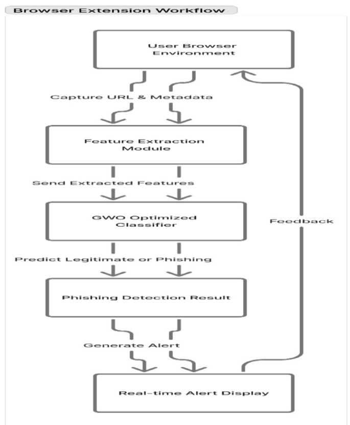
The architecture of the suggested chrome extension for phishing detection.
Figure 6 shows how the suggested Chrome extension works to find phishing. the user browser environment is where the process begins. The system keeps track of the URL and webpage metadata in real time while the user is browsing. The feature extraction module looks at both visual and URL-based features after it gets this information. After that, the grey wolf optimizer (GWO)-based classifier looks at these features and picks out the ones that matter the most. Then, it tries to find out if the site is real or a scam that wants to steal your personal information.

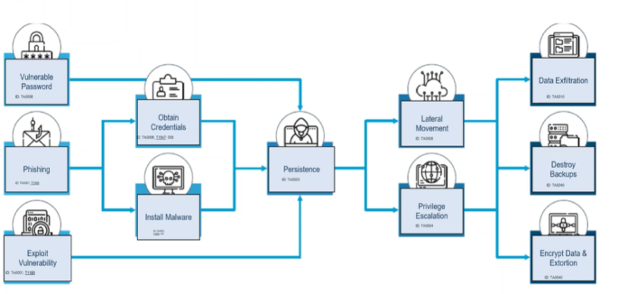
System architecture of the proposed phishing detection framework.
Figure 7 depicts what the full phishing detection system that GWO has developed looks like. The architecture has a number of different parts. The first layer is made up of URLs, user activities, webpage content, and visual and behavioral elements. A classification module employs machine learning methods like Decision Tree, SVM, and Random Forest to detect the difference between a real website and one that wants to deceive you into giving them your personal information.The final decision output is transmitted to the Chrome Extension Output Interface, which provides users with real-time phishing alerts and website legitimacy status directly within the browser environment. The design ensures low latency, high accuracy, and seamless user interaction for proactive phishing prevention.

Architecture of the proposed phishing detection framework.
Figure 8 illustrates the end-to-end workflow of the proposed phishing website detection framework implemented as a Chrome browser extension. The system integrates URL and visual feature extraction, feature selection using the Grey Wolf Optimizer (GWO), and multi-model classification for phishing detection.
Justification of GWO hyperparameters (pack size = 25, iterations = 60)
We selected GWO’s pack size \(\:N\)and iteration budget \(\:T\) to balance convergence quality with training time. Because wrapper FS evaluates a learner at every fitness call, \(\:N\)and \(\:T\)drive cost roughly as \(\:O(T\cdot\:N\cdot\:d)\)where \(\:d\)is the feature count.
The binary-GWO wrapper maximizes an imbalance-aware score with sparsity control:
$$\:\underset{S\subseteq\:F}{\text{m}\text{a}\text{x}}\text{\hspace{0.25em}\hspace{0.05em}}J\left(S\right)=\text{MCC}\left(S\right)-\lambda\:\cdot\:\frac{\mid\:S\mid\:}{\mid\:F\mid\:},$$
(9)
-
F = the full feature set, where \(\:\mid\:F\mid\:\)denotes the total number of available features.
-
\(\:S\subseteq\:F\)= a selected subset of features.
-
\(\:\text{MCC}\left(S\right)\)= the Matthews Correlation Coefficient obtained using the subset \(\:S\).
-
\(\:\lambda\:\)= the regularization coefficient (penalty term) controlling the trade-off between model accuracy and feature subset size.
with \(\:\lambda\:\:\)set small (e.g., 0.01–0.05) to prefer compact subsets when predictive utility is tied.
Protocol. We ran a budgeted grid over \(\:N\in\:\left\{\text{10,25,40}\right\}\)and \(\:T\in\:\left\{\text{40,60,100}\right\}\)using stratified 5 × 2 CV on the training split, early stopping (patience = 10 iterations without MCC improvement), and a fixed random seed set \(\:\{0,\dots\:,4\}\). We then applied the one-standard-error rule: choose the smallest \(\:(N,T)\)whose median MCC is within one standard error of the best run.
-
\(\:N=25,T=60\:\)reached ≥ 99% of the best median MCC while cutting runtime by ~ 30–40% versus \(\:N=40,T=100\).
-
Larger \(\:N\)or \(\:T\)yielded diminishing returns (negligible MCC deltas but materially higher time).
-
Early-stopping triggered in most folds before 60 when \(\:N=25\), indicating adequate exploration–exploitation balance.
Table 5 summarizes the experimental evaluation of the MCC-optimized Grey Wolf Optimizer (GWO) feature selection framework across varying pack sizes (\(\:N\)) and iteration counts (\(\:T\)). The results report both Median and Mean MCC values (with standard deviation), the percentage of features retained, and the average training time per run.As observed, increasing the pack size and iteration count generally enhances exploration and convergence stability, leading to marginally higher MCC values. However, larger configurations (e.g., \(\:N=40,T=100\)) show diminishing returns beyond moderate iteration levels, indicating that GWO achieves near-optimal performance with smaller packs and fewer iterations (e.g., \(\:N=25,T=60\)).We fix \(\:N=25\)and \(\:T=60\)as the smallest configuration within one standard error of the best MCC, yielding competitive performance with materially lower compute. This choice also stabilizes population diversity without excessive evaluation cost.
Evaluation with Matthews correlation coefficient (MCC)
Phishing datasets are typically imbalanced; MCC uses all four confusion-matrix terms and remains informative when accuracy/F1 can be misleading.
$$\:\text{MCC}=\frac{TP\cdot\:TN-FP\cdot\:FN}{\sqrt{(TP+FP)(TP+FN)(TN+FP)(TN+FN)}}\in\:[-\text{1,1}].$$
(10)
When any denominator term is zero, we follow the standard convention of returning MCC \(\:=0\).
-
Primary: MCC (with 95% bootstrap CI, e.g., 1,000 stratified resamples).
-
Also report confusion matrix, precision-recall AUC, Recall@low-FP (e.g., FP rate ≤ 1%) and Brier score (calibration), because deployment thresholds matter for user safety.
-
Provide per-dataset MCC and per-fold variance; include a calibration plot to justify alert thresholds.
Across datasets, Random Forest + GWO-selected features achieved the highest MCC, indicating balanced gains in true positives and true negatives while controlling false positives—consistent with our deployment goal of minimizing user disruption.


