Water quality index prediction via a robust machine learning model using oxygen-related indices for river water quality monitoring

Study area

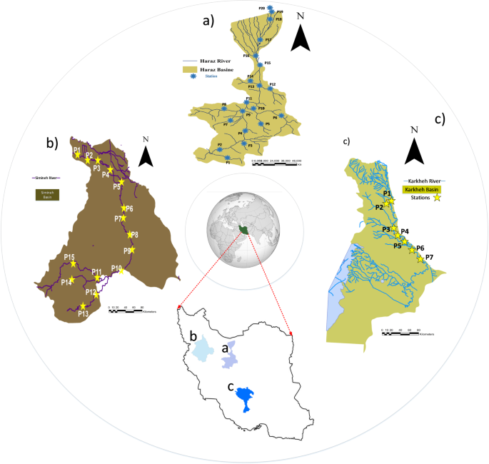
This study focuses on three major rivers in Iran, the Karkheh, Haraz, and Simineh, which were strategically selected to serve as a robust testbed for model development and validation (Fig. 1). The primary justification for their selection is their significant diversity in hydro-climatic and environmental conditions. The Karkheh River flows through semi-arid regions, the Haraz is situated in a temperate, mountainous area, and the Simineh drains a sub-catchment of the environmentally sensitive Lake Urmia watershed. This diversity provides a wide spectrum of water quality conditions, making it an ideal setting to develop a single, universally applicable “Super Model” and rigorously test its ability to generalize across different ecosystem types, a core objective of this research.

The Karkheh River, the third-longest river in Iran after the Karun and Sefidroud rivers, originates from the Zagros Mountains and flows through the northern part of Khuzestan, particularly near Pol-Zal. The river is formed by the confluence of the Pol-Zal and Seymare rivers near Andimeshk and Susa. largest dam in Iran, the Karkheh Dam, is located on this river¹⁹. The Karkheh basin experiences a wide range of climatic conditions, with temperatures recorded from − 25 °C to + 50 °C. The basin has a Mediterranean climate, with an average annual precipitation of approximately 290.6 mm at the dam site, and a mean annual temperature of about 24.6 °C, with recorded extremes of 53.6 °C and − 4.2 °C.

The Simineh River basin is a significant sub-catchment of the Lake Urmia watershed, located in the northwestern parts of Iran, specifically in the West Azerbaijan and Kurdistan provinces²⁰. The river originates from the highlands south and southwest of Saqqez County, flowing through mountainous terrain and plains before entering the Miandoab plain and eventually draining into Lake Urmia. The basin exhibits notable topographic and climatic diversity, with elevations ranging from 1,352 m at the headwaters to approximately 1,200 m in the Miandoab plain. The basin encompasses parts of Saqqez, Bukan, Mahabad, and Miandoab counties, covering an area of 3,787 km². Geologically, the basin is characterized by carbonate and non-carbonate sedimentary formations, as well as volcanic and metamorphic units. Land use in the area is dominated by agriculture, with the remainder consisting of rangelands, forests, and human settlements. The Simineh River is crucial for drinking water, irrigation, and groundwater recharge, although it faces challenges from urban expansion, industrial discharges, and agricultural runoff, which have significantly degraded its water quality. Consequently, the Simineh River basin is an important case study in water resource management and environmental challenges in semi-arid regions of Iran.

The study area also includes the northern part of Iran, covering a significant portion of the southern coastal plain of the Caspian Sea. This region is defined by the watersheds of the Haraz, Garmarud, and Babolrud rivers. Geographically, the area extends from the Caspian Sea coastline in the north to the central Alborz mountain range in the south. The Haraz River system dominates the hydrology of the region, originating from Mount Damavand and draining a watershed of approximately 4,000 km². Two main tributaries of river, the Noor and Lar rivers, converge south of Amol, and the river flows northwards into the Caspian Sea. The region is water-rich²¹, characterized by a high density of rivers and streams fed by mountain precipitation and snowmelt, although seasonal flow variations are significant. The region is water-rich, characterized by a high density of rivers and streams fed by mountain precipitation and snowmelt, although seasonal flow variations are significant. Annual precipitation averages around 770–850 mm, with the highest levels occurring in autumn and winter. The average annual temperature is approximately 14.1 °C, with clear seasonal variations, the warmest month being August and the coolest being February, Relative humidity is consistently high, contributing to the region’s lush vegetation.

Human activities have significantly shaped the landscape, with agriculture covering approximately 46.1% of the area, predominantly in the fertile coastal plains. Forests make up 29.6% of the land, mainly in the southern mountainous areas, while mixed-use zones of agriculture and orchards account for 18.3%. Urban areas occupy 3.5%, and ecologically significant water reservoirs known as Ab-bandans cover 1.1% of the study area.

Field procedures and In-Situ measurements

The training dataset for the SVR “Super Model” was sourced from an intensive monitoring program on the Karkheh River. Monthly water samples were systematically collected from January 2022 to November 2022 at seven strategically selected stations. This 11-month period provided a comprehensive dataset covering a full range of seasonal variations. In total, 77 samples (7 stations × 11 months) were collected and analyzed, forming the basis for training the model²².

The first independent validation dataset was from the Haraz River basin. Data were collected in a single, comprehensive sampling campaign across 20 strategically chosen stations. This resulted in a total of 20 samples, providing a spatially diverse snapshot for the first validation test.

The second validation dataset was from a monitoring program on the Simineh River. Sampling was conducted seasonally at 15 primary stations over a one-year period, comprising a total of four sampling rounds (one per season). This resulted in a dataset of 60 samples (15 stations × 4 rounds), offering a temporally representative dataset to test the model’s generalization capabilities across different seasonal conditions.

The reliability of the water quality assessment in this study was heavily reliant on a meticulously planned sampling and measurement protocol. Monthly water samples were collected from January to November across twenty strategically chosen stations. To minimize the effects of diurnal fluctuations, especially concerning DO levels, all in-situ measurements were consistently conducted between 08:00 and 10:00 AM²³. At each station, key physicochemical parameters, including water temperature (T_w), DO, EC, and pH, were measured in-situ using a calibrated YSI ProDSS multi-parameter probe²⁴. These measurements were performed before the collection of physical water samples to ensure the data reflected undisturbed, natural stream conditions.

Instrument accuracy was maintained through daily calibration protocols, performed each morning before deployment, using certified standard solutions, in line with manufacturer specifications (e.g., WTW Multi 340i/SET, HORIBA Checker V-10). To improve sample representativeness and minimize surface-level biases, water samples were taken from the mid-depth of the water column (approximately 50% of the total depth) using a Van Dorn horizontal sampler²⁵. For increased accuracy and reproducibility, all in-situ measurements were performed in triplicate, with the average value used for subsequent data analysis.

The integrity of the water quality values (WQVs) assessment relied on the precision of the sampling and measurement procedures. Monthly water samples were systematically collected from January 2021 to November 2022 at seven strategically selected stations along the River. These stations represented the micro-basins of the upstream reach, where land-use changes, point-source discharges, and flow rates exhibit minimal variation. A total of 77 samples were collected over the 11-month period. Sampling occurred on the first Monday of each month, between 06:00 and 10:00 AM, to reduce interference from daylight variations, particularly concerning DO concentrations, which are affected by photosynthetic processes²³.

At each station, in-situ measurements of core physicochemical parameters (T, DO, EC, and pH) were conducted using a calibrated YSI ProDSS multi-parameter probe²⁴. To ensure unbiased sampling, water samples were collected from the mid-depth of the river, approximately 50% of the total water column depth, using a Van Dorn horizontal sampler. Additionally, river velocity was measured using a Molina propeller meter (number 4), which has an accuracy of 0.06 and can detect flow rates of up to 5 m/s²⁴. To minimize human error in water height (H) measurements, a two-person system was implemented, where both individuals took measurements simultaneously from a perpendicular angle to the water surface.

The monitoring network for the Simineh River was strategically designed to capture spatio-temporal dynamics in water quality across the basin. A total of 15 primary sampling stations were established, extending from the upstream headwaters to the downstream reaches near Miandoab. Station selection followed a multi-criteria approach, prioritizing locations based on key hydrological features (e.g., confluences with major tributaries and sites upstream and downstream of urban centers like Bukan and Miandoab), pollution sources (e.g., downstream of point sources such as the Bukan Wastewater Treatment Plant and non-point sources like agricultural drainage), and logistical considerations for seasonal accessibility and safety.

Sampling was conducted seasonally in four campaigns to capture variability across different hydrological conditions, such as high-flow spring and low-flow autumn. In-situ physicochemical parameters, including T, DO, pH, and EC, were measured at each station using calibrated portable multi-parameter probes (e.g., Crison OXI 45, Hach DR/4000 Spectrophotometer). Water samples for laboratory analysis were collected from the main thalweg at mid-depth to ensure representativeness and avoid surface or benthic biases²⁶. This robust sampling framework enabled a comprehensive analysis of pollution transport, attenuation, and self-purification processes within the river system.

Sample Preservation, Transport, and quality assurance

To maintain the integrity of water samples from collection through to laboratory analysis, stringent preservation and handling procedures were adhered to, following established protocols, including those from the U.S. Environmental Protection Agency (EPA) Region 4 and standard environmental guidelines. Immediately after collection, samples were transferred into pre-cleaned polyethylene bottles and stored in portable iceboxes at approximately 4°^C to minimize biological and chemical activity. This temperature control helped preserve reactive parameters such as nutrients and biochemical oxygen demand (BOD₅). Samples were then transported to the laboratory within 24 h to prevent degradation, ensuring they remained within the prescribed holding times to avoid any changes that could affect the analysis²⁷.

Quality assurance and quality control (QA/QC) measures were systematically followed throughout the sampling and transport processes. This included the use of field duplicates to evaluate sampling precision, equipment blanks to check for contamination, and detailed documentation of sampling conditions, including the time, weather, and visual observations. A chain-of-custody protocol was also maintained to ensure sample traceability and preserve the integrity of the data from collection through to analysis. Field activities were meticulously documented, ensuring full transparency and defensibility of the study’s findings²⁸.

Laboratory analytical methods and quality control

Once received in the laboratory, water samples were analyzed using internationally recognized methods to ensure consistent and reliable results. These analyses included gravimetric methods for Total Solids (TS), Total Suspended Solids (TSS), and Total Dissolved Solids (TDS), spectrophotometric methods for nutrients like Nitrate-Nitrogen (NO₃-N) and Orthophosphate (PO₄-P), as well as the BOD₅²⁹ test and microbiological analysis for Total Coliforms (TC) and Fecal Coliforms (FC).

All laboratory analyses followed the procedures outlined in the Standard Methods for the Examination of Water and Wastewater (APHA, 2023), ensuring methodological consistency and comparability. Specific methods included:

• Nutrient analysis using a Seal AQ2 discrete analyzer with detection limits of 0.01–0.05 mg/L.

• Atomic absorption spectrophotometry using a Varian Specter AAA 400 for metal analysis.

• Turbidity measured by a Hach 2100 N turbidimeter.

• TSS determined through gravimetric analysis following Standard Method 2540D.

• BOD₅ measured through the 5-day incubation method at 20 °C.

For quality control, all samples were analyzed in duplicate to assess precision and accuracy. Regular calibration of instruments with certified standards, analysis of method blanks, and use of matrix spikes helped assess analytical recovery and identify any potential interference in the samples. Additional QA/QC measures included external checks, field duplicates analyzed by independent teams, and split samples for comparison with outside laboratories for validation.

A comprehensive Quality Assurance Project Plan (QAPP) was developed to outline all procedures, ensuring high data quality. Field blanks, lab replicates, spike samples, and calibration blanks were incorporated throughout the study to further verify the reliability of the measurements and minimize errors in the analytical process. These rigorous measures were implemented to uphold the integrity of the study and ensure the accuracy of the results.

Initial assessment of datasets and preliminary correlation analysis to explore parameter relationships

Prior to model training, the consolidated dataset from the Karkheh River underwent a critical preprocessing phase to ensure the optimal performance of the SVR algorithm. This step is essential because SVR is sensitive to the scale and range of the input features; variables with larger magnitudes can disproportionately influence the model’s learning process.

To address this, all input features, DO, BOD, COD, and Water Temperature, were standardized using the Z-score method (Eq. 1). This technique rescales each feature so that it has a mean (µ) of 0 and a standard deviation (σ) of 1. The transformation for each data point x is calculated as:

The initial assessment of the water quality dataset aimed to understand its inherent structure, variability, and inter-relationships among the measured hydrochemical parameters before proceeding to detailed modeling. Descriptive statistics, including mean, median, standard deviation, minimum, maximum, and range, were first calculated for all parameters to examine data distributions, detect extreme values, and identify missing or censored observations. Missing values and censored data (e.g., values reported as < 1) were appropriately imputed or replaced to maintain numerical consistency.

To visualize the overall structure of the multi-dimensional dataset, Uniform Manifold Approximation and Projection (UMAP) was applied, reducing the dataset to a two-dimensional representation³⁰. This approach facilitated the identification of intrinsic patterns and potential clusters, revealing similarities and differences among the sampling sites and rivers.

Outlier detection was performed using a One-Class Support Vector Machine (SVM), complemented by standardized Z-scores computed for each parameter³¹. Heatmaps of these standardized scores were generated to visualize parameter-wise deviations and identify anomalous samples, ensuring that extreme values did not bias further statistical or modeling procedures. In addition, one-way ANOVA was conducted to statistically evaluate differences between inlier and outlier groups, computing F-statistics and p-values for each parameter to identify variables that contributed most to water quality variability³².

Collectively, these analyses provided a comprehensive understanding of the dataset’s structure, inter-parameter relationships, and anomalous observations, laying a robust foundation for subsequent ecological interpretation and predictive modeling of water quality dynamics.

Developing a WQI_OIs prediction model using Oxygen-Related indices

Recognizing DO as the paramount indicator of aquatic ecosystem health, we developed a predictive model for the WQI_OIs centered on DO dynamics and its key influencing factors. A Support Vector Regression (SVR) model³³ was selected as the core predictive engine due to its proven efficacy in capturing complex, non-linear relationships, which are characteristic of environmental systems. The development process was structured to create a robust, generalizable, and interpretable model.

The predictive power of an SVR model is highly dependent on the selection of its key hyperparameters. For this study, which utilized the common and effective Radial Basis Function (RBF) kernel, three primary hyperparameters were optimized: C, γ (gamma), and ε (epsilon).

• The Regularization Parameter (C): This parameter controls the trade-off between achieving a low training error and minimizing model complexity (i.e., keeping the decision surface smooth). A high value of C places a large penalty on training errors, forcing the model to fit the training data as closely as possible, which can lead to overfitting. Conversely, a low value of C allows for a larger margin and tolerates more errors, which can lead to a simpler model that may underfit the data.

• The Kernel Coefficient (γ): The gamma parameter defines how much influence a single training example has. A high gamma value means the influence is local, leading to a more complex, “wiggly” decision boundary that can also result in overfitting. A low gamma value means the influence is far-reaching, resulting in a much smoother, more generalized decision boundary that can lead to underfitting.

• The Epsilon (ε) Parameter: This parameter defines the width of the “epsilon-insensitive tube” around the regression function. Any data points that fall within this tube are considered to have zero error and do not contribute to the regression loss. It essentially sets a margin of tolerance for errors. A larger ε results in a wider tube and fewer support vectors, leading to a simpler, more generalized model. A smaller ε results in a narrower tube, tolerating less error and potentially creating a more complex model.

Feature selection and engineering

The predictive model was developed using a set of input features selected for their direct or indirect influence on oxygen dynamics in rivers. DO (mg/L) was incorporated as the primary response variable, while BOD₅ (mg/L) and COD (mg/L) were included as key indicators of oxygen consumption. T_w (°C) was considered the main environmental driver, given its strong control over both solubility and reaction kinetics. To further embed process-based knowledge into the modeling framework, T_w values were used to derive the K₁, providing a physics-informed parameter that reflects the temperature-dependent kinetics of oxygen depletion. This combination of measured and derived features ensured that the model captured both the empirical variability and the mechanistic processes governing oxygen status in the studied rivers. This was calculated using the standard thermal correction equation (\(\:{K}_{1}\left(T\right)=0.3\times\:{1.047}^{(T-20)}\)), thereby transforming a simple temperature measurement into a biologically meaningful rate of oxygen consumption. This feature engineering step ensures the model is not only data-driven but also grounded in established immunological principles.

Model training and generalization

To develop a single, universally applicable model rather than one calibrated to a specific location, a “Super Model” was trained. The training dataset was a comprehensive consolidation of all available data from the river system under study (Karkheh River). This approach exposes the SVR algorithm to a wide spectrum of hydro-chemical conditions, forcing it to learn the fundamental relationships between the input features and the WQI_OIs, rather than memorizing the specific characteristics of a single river. This strategy is explicitly designed to enhance the model’s generalization capability, its ability to make accurate predictions on new, previously unseen data.

Model interpretability using SHAP, enrichment Plot, confusion matrix and

A central tenet of this work is to move beyond “black-box” predictions. To ensure transparency and build confidence in the model’s internal logic, we employed SHAP (SHapley Additive exPlanations). SHAP is a state-of-the-art, game theory-based approach that calculates the contribution of each feature to each individual prediction. By analyzing the SHAP values across the dataset, we can determine not only the global importance of each feature but also understand how the value of a feature (e.g., a high vs. low DO measurement) influences the final WQI_OIs output. This provides a rigorous, quantitative method to verify that the model’s decision-making process aligns with established ecological knowledge³⁴.

A method called Feature Set Enrichment Analysis (FSEA), based on Enrichment Analysis (EA), was developed to check if specific sets of samples are linked to degraded water quality conditions. Unlike simple correlation, this method looks at how a feature set is distributed across the full range of water quality.

The FSEA procedure was as follows:

• Ranked List Generation: All samples from the consolidated dataset were ordered into a single list, ranked from highest (best quality) to lowest (worst quality) based on the WQI_OIs predicted by the validated SVR Super Model. This creates a continuous quality gradient that serves as the basis for the analysis.

• Definition of the Feature Set: A set of interest was defined based on a key environmental characteristic. For this study, the “Hot Samples” set were defined, comprising all samples recorded during the hot season (Temperature ≥ 20 °C).

• Enrichment Score Calculation: An Enrichment Score (ES) was calculated by walking down the ranked list from top to bottom. The ES starts at zero and is increased for every sample encountered that belongs to the “Hot Samples” set (a “hit”) and decreased for every sample that does not (a “miss”). The magnitude of the increase is inversely proportional to the number of hits, and the magnitude of the decrease is inversely proportional to the number of misses.

• Visualization: The resulting ES profile was plotted, along with a “barcode” view showing the precise location of the “Hot Samples” within the ranked list. A significant, non-random distribution is indicated by a peak in the ES at either end of the ranked list.

To evaluate the ability of model to accurately categorize water quality into practical management classes, its performance as a multi-class classifier was assessed. All WQI_OIs were assigned to one of four classes: ‘Poor’, ‘Moderate’, ‘Good’, or ‘Excellent’. The continuous WQI_OIs score predicted by the SVR model was then used to assign a predicted class to each sample using the same thresholds. The classification of model accuracy was then visualized using a Confusion Matrix. This matrix provides a detailed breakdown of performance by showing the counts of correct predictions (on the diagonal) and incorrect predictions (off-diagonal) for each class, allowing for an in-depth analysis of the model’s specific strengths and weaknesses in categorizing ecosystem health.

To quantify the model’s ability to discriminate between pristine and impacted water quality states, a Cumulative Accuracy Profile (CAP) analysis was performed. This is a standard technique for evaluating the discriminatory power of a scoring classifier.

The continuous WQI_OIs score predicted by the SVR model was used to rank all samples from lowest to highest. The CAP curve was then generated by plotting the cumulative percentage of positive-class samples identified against the cumulative percentage of the total sample population. The model’s curve was compared against a theoretical “Perfect Model” and a “Random Model” baseline to assess its performance. The Accuracy Ratio (AR) was calculated as the primary quantitative metric of discriminatory power.

Aplicability of WQI_OIs on Haraz river and Simineh river

To rigorously evaluate the generalization capability and practical applicability of the trained Super Model, a validation protocol was conducted on two independent river datasets not used during the initial model development phase: The Haraz River and the Simineh River. For both datasets, the requisite input features corresponding to the simplest and most universally available model configuration, namely DO and T_w, were extracted. Consistent with the methodology described in Sect. 2.6.1, the T_w data was further utilized to calculate the derived K₁, thereby generating two distinct and unseen test sets.

The trained Super Model was subsequently applied to produce WQI_OIs predictions for all samples within these datasets. To provide a credible scientific benchmark for comparison, a standardized, equation-based WQI_OIs was also computed for each sample using the Weighted Geometric Mean methodology (Said et al., 2004). This established index integrates a broader suite of measured hydrochemical parameters, including DO, BOD₅, pH, nitrates, and phosphates—and is widely recognized in the water quality literature as a robust and comprehensive reference. Thus, this parallel calculation enabled a direct comparison between the machine learning–based predictions³⁵, developed with a streamlined feature set, and a conventional, multi-parameter index.

The applicability of the model was assessed primarily through the Pearson correlation coefficient (r), calculated between the SVR model predictions and the benchmark WQI_OIs values for each river independently. A strong positive correlation (with r values approaching 1.0) was interpreted as evidence that the model, despite its reduced feature requirements, successfully reproduced the temporal patterns, fluctuations, and overall dynamics of water quality captured by the benchmark index. This outcome would provide robust support for the capacity of model to deliver directionally accurate and scientifically meaningful assessments across new and unseen river systems, thereby underscoring its potential utility as a monitoring and decision-support tool.

Preventing overfitting—where a model memorizes training data noise instead of learning true patterns—was a primary methodological concern. To mitigate this risk, a multi-faceted strategy was employed. The model’s key hyperparameters (C, γ, ε), particularly the regularization parameter C which directly controls complexity, were optimized using a systematic Grid Search coupled with a robust 10-fold cross-validation procedure. This process inherently penalizes models that do not perform consistently across different subsets of the data, preventing the selection of an overly complex model. However, the most definitive test of the model’s robustness was its final evaluation on two completely independent and unseen river datasets (Haraz and Simineh). The model’s high predictive accuracy on this new data provides the strongest possible evidence that it successfully learned generalizable, underlying relationships rather than overfitting to the training set, thereby ensuring its reliability for practical applications.