Ethics statement
This study exclusively used publicly available datasets. No new human or animal samples were collected, and no experiments involving human participants or animals were performed by the authors. Therefore, ethical approval was not required for this study. Sex and/or gender was not considered in the study design or analysis, as this work focuses on computational method development rather than biological comparisons between sexes or genders, and sex- or gender-disaggregated information was not consistently available across the public datasets used.
Data
Simulated data were generated using the method outlined by Townes et al.41, which is designed to produce synthetic datasets with specific spatial structures, facilitating the validation of the model’s ability to identify and process spatial features effectively. The simulation generated multivariate counts with spatial correlation patterns. We use the ggblocks simulation which is based on the Indian Buffet Process, where each latent factor represents a typical spatial pattern defined over a 36 × 36 grid of locations (\(N=1296\) spatial locations). For the RNA and ATAC modalities, we generated spatial expression matrices of size 1296 cells × 1000 genes (peaks) characterized by four factors and following a zero-inflated negative binomial distribution (ZINB). For the protein modality, we generated a spatial expression matrix of size 1296 cells × 100 proteins characterized by four factors and following a negative binomial distribution (NB). The negative binomial distribution introduces randomness by modeling the variability of discrete events. This variability is considered noise, representing the uncertain portion of the data and simulating the random fluctuations observed in real-world data.
10x Genomics CytAssist Visium datasets were generated using the 10x Genomics CytAssist Visium platform, which enables the joint profiling of transcriptome and protein expression. They include the human lymph node dataset used in SMART for spatial transcriptomics and proteomics integration, and the three-section tonsil dataset used in SMART-MS for multi-section integration. This platform integrates spatial whole-transcriptome sequencing with multiplexed protein detection on a single tissue section via next-generation sequencing (NGS), with a spatial resolution of 55 µm, a spot spacing of 100 µm, and an imaging area of 6.5 mm × 6.5 mm. The lymph node dataset consists of two tissue sections: Human Lymph Node A1 (3484 spots) and D1 (3359 spots), each containing expression profiles of 18,085 genes and 31 proteins. The tonsil dataset includes three sections with 4326, 4519, and 4521 spots, respectively. Each section contains 18,085 genes; the first two sections include 31 proteins, while the third section includes 35 proteins.
MISAR-seq mouse brain datasets were generated by measuring spatial transcriptome and chromatin accessibility in the mouse brain using MISAR-seq², a microfluidic indexing–based spatial assay for transposase-accessible chromatin and RNA sequencing. MISAR-seq enables spatially resolved joint profiling of chromatin accessibility and gene expression. In this dataset, the tissue is positioned on a microfluidic chip, where a grid-based spatial barcoding system assigns unique DNA barcodes across 2500 grids, each 50 × 50 µm, covering approximately 5–20 cells per grid. This dataset includes eight sections of the mouse fetal brain at embryonic days, i.e., E11.0, E13.5, E15.5, and E18.5. The number of grids covered by the sections ranges from 1263 to 2248, with a total of 32,285 sequenced genes and peak counts varying from 60,112 to 143,879.
Spatial Epigenome–Transcriptome mouse brain datasets originate from the method proposed by Zhang et al.1, including spatial ATAC–RNA-seq and CUT&Tag–RNA-seq, which enable simultaneous detection of chromatin accessibility or histone modifications (e.g., H3K27me3, H3K27ac, or H3K4me3) together with gene expression within a single tissue section at near single-cell resolution. In the P22 mouse brain coronal sections, a 100 × 100 barcode grid (pixel size: 20 µm) was used to cover the entire hemisphere region, with most pixels capturing 1–3 cells. The RNA + H3K27me3 dataset used to evaluate the scalability of SMART contains 9752 spots, 70,470 peaks, and 25,881 genes. Meanwhile, the RNA + ATAC dataset used to assess multi-section integration with SMART-MS includes three sections with 2372, 2497, and 9215 spots, respectively, along with 161,514 peaks and 18,107 genes.
STARmap-RIBOmap-Align datasets were generated by applying STARmap, a high-resolution spatial transcriptomics technology developed by Wang et al.46, and RIBOmap, a three-dimensional in situ spatial translatomics method introduced by Zeng et al.47, to consecutive mouse brain tissue sections, enabling joint measurement of transcriptomic and translatomic profiles for 5,413 genes at single-cell and molecular resolution. The STARmap section contained 59,165 spots, and the RIBOmap section contained 58,692 spots. Using the CAST projection algorithm introduced by Tang48, spots from the STARmap section were aligned to those in the RIBOmap section, resulting in dual-omics data for 58,692 spots.
The SPOTS mouse spleen dataset was generated using Spatial PrOtein and Transcriptome Sequencing (SPOTS)⁴ to profile spatial transcriptomic and proteomic data for assessing multi-section integration with SMART-MS. Similar to 10X Human Lymph Node dataset, SPOTS also offers a spatial resolution of 55 µm, with a distance of 100 µm between spots, covering an imaging area of 6.5 mm × 6.5 mm. This dataset includes two sections, SPOTS Spleen Replicate 1 and SPOTS Spleen Replicate 2, containing 2647 and 2759 spots, respectively, with each section capturing the expression of 32,285 genes and 21 antibody-derived tags (ADTs).
Stereo-CITE-seq datasets were generated using the method proposed by Liao et al.6, which combines CITE-seq with Stereo-seq to enable simultaneous profiling of the transcriptome and proteome on the same tissue section at subcellular spatial resolution (0.5 µm) with high reproducibility and precision. This technique achieves a spatial resolution of up to 0.22 µm, with a spot spacing of 0.5 µm and an imaging area of 200 mm². The mouse spleen dataset used to evaluate the scalability of SMART was processed into multiple resolution levels, including Bin10 (5 µm), Bin20 (10 µm), Bin50 (25 µm), Bin100 (50 µm), Bin150 (75 µm), and Bin200 (100 µm), comprising 756,430; 189,867; 30,652; 7,782; 3507; and 2001 spots, respectively. In addition to spot-level representations generated by spatial binning, we also used the image-guided cell segmentation results provided by the Stereo-CITE-seq pipeline (cellbin.gef), in which RNA and protein signals are aggregated at the single-cell level. These data were used to evaluate SMART’s applicability to single-cell–segmented spatial data. This dataset includes expression data for 29,034 genes and 128 ADTs. For evaluating multi-section integration with SMART-MS, we used three mouse thymus sections at Bin50 resolution (25 µm), which contain 4253, 4646, and 4228 spots, respectively. Each section captures expression profiles for 23,221 to 23,960 genes and 19 ADTs.
Data preprocessing
Spatial transcriptomic data were preprocessed by first removing genes expressed in fewer than 10 spots to minimize the impact of low-abundance signals. The top 3000 or 5000 highly variable genes were then selected to retain features contributing most to data variability. Expression counts were normalized by scaling the total expression in each spot to 10,000 to account for differences in sequencing depth, followed by logarithmic transformation to reduce the influence of highly expressed genes and approximate a normal distribution. The data were subsequently scaled to zero mean and unit variance.
Spatial chromatin accessibility data were preprocessed by first applying a TF–IDF transformation to accessible chromatin regions, with a scaling factor of 10,000 to downweight commonly accessible regions and emphasize features with higher variability across spots. Peak counts within each spot were then normalized by scaling the total signal to 10,000 to correct for differences in sequencing depth. A logarithmic transformation was subsequently applied to stabilize variance and reduce the influence of highly accessible regions, preparing the data for downstream analyses.
Spatial protein data were preprocessed by first applying a centered log-ratio transformation to remove scale differences across proteins. The data were then standardized to zero mean and unit variance to ensure that all protein features were on a comparable scale for downstream analyses.
The SMART framework
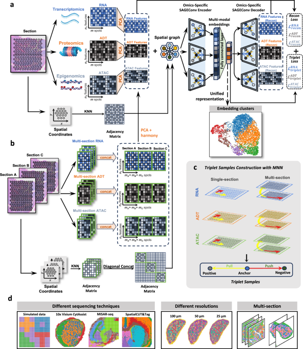
SMART is a deep learning model that leverages graph neural networks and metric learning to integrate spatially-resolved multi-modal omics into unified embeddings. For each modality, SMART extracts principal components (PCs) using principal component analysis (PCA) and constructs spatial neighboring graphs with PCs as node features. Spatial graphs are built based on the coordinates of spatial units using a k-nearest-neighbor (kNN) strategy. In spot-based analyses, nodes correspond to spots or bins, whereas in single-cell–segmented analyses, nodes correspond to individual cells, with cell centroids used as spatial coordinates. For single-cell–segmented data, radius within one cell distance to select the nearest cells around can also be used in spatial graph construction. Then, the model employs SAGEConv (Sample and Aggregate Convolution) to aggregate both the spatial information and the PCs from a specific modal omics, thereby synthesizing a integrate representation of the omics. Ultimately, these representations are combined into a unified intermodal embedding.
However, using spatial neighboring graphs for aggregation may neglect the feature correlations even in long distance. Therefore, we further adjust the graph aggregation using metric learning with triplet loss to ensure the mutual correlation between spots or bins in the original omics. The loss functions of reconstruction to the original omics and the triplet loss are crucial to guarantee the representation of the original omic intact after embedding with spatial information.
In a spatial multi-omics dataset featuring three distinct omics modalities, the inputs to SMART consist of characteristics for each modality \({{{{\bf{X}}}}}_{1}\in {{\mathbb{R}}}^{m\times {n}_{1}},{{{{\bf{X}}}}}_{2}\in {{\mathbb{R}}}^{m\times {n}_{2}}\), and \({{{{\bf{X}}}}}_{3}\in {{\mathbb{R}}}^{m\times {n}_{3}}\) and the spatial coordinates \(S\in {{\mathbb{R}}}^{m\times 2}\). Here \(m\) represents the number of spots in the tissue section, while \({n}_{1},{n}_{2}\), and \({n}_{3}\) correspond to the number of features in the three omics modality, for example, the number of genes in transcriptome. In the simulated spatial multi-omics data, \({{{{\bf{X}}}}}_{1}\), \({{{{\bf{X}}}}}_{2}\), and \({{{{\bf{X}}}}}_{3}\) represent the features of transcriptome, proteome, and epigenome. The output of SMART is a unified embedded representation \({{{{\bf{Z}}}}{\mathbb{\in }}{\mathbb{R}}}^{N\times f}\) in the low-dimensional latent space, which integrates information from multiple spatial omics. The parameter \(f\) is denoted as the dimension in the latent space. If there are two omics, the inputs become \({{{{\bf{X}}}}}_{1}\in {{\mathbb{R}}}^{m\times {n}_{1}},{{{{\bf{X}}}}}_{2}\in {{\mathbb{R}}}^{m\times {n}_{2}}\) and the rest of the operation is the same. Overall, the main components of SMART can be categorized into five modules: principal component analysis, spatial neighboring graph construction, SAGEConv encoder, triplet construction, and SAGEConv decoder. Each module is elaborated in the following sections.
Principal component analysis
We first apply PCA to the preprocessed data from each modality: \({{{{\bf{X}}}}}_{1}\in {{\mathbb{R}}}^{m\times {n}_{1}},{{{{\bf{X}}}}}_{2}\in {{\mathbb{R}}}^{m\times {n}_{2}}\), and \({{{{\bf{X}}}}}_{3}\in {{\mathbb{R}}}^{m\times {n}_{3}}\), in order to reduce the dimensionality of the data to \({d}_{1}\), \({d}_{2}\) and \({d}_{3}\) dimensions, respectively. Specifically, after applying PCA, we obtain the dimensionality-reduced feature matrices: \({{{{\bf{X}}}}}_{1}\in {{\mathbb{R}}}^{m\times {d}_{1}},{{{{\bf{X}}}}}_{2}\in {{\mathbb{R}}}^{m\times {d}_{2}}\) and \({{{{\bf{X}}}}}_{3}\in {{\mathbb{R}}}^{m\times {d}_{3}}\). By retaining the most representative principal components, we achieve the dimensionality reduction. Typically, the dimensionality of the transcriptomics and chromatin accessibility modalities is reduced to 30, while the dimensionality of the proteomics modality is determined based on the number of ADTs.
Spatial neighboring graph construction
To learn the spatial coordination of omics, we constructed a spatial neighboring graph with each spot or bin as node and principal components as node feature. Each node (spot or bin) was connected to its \({{{\rm{k}}}}\) nearest neighbors according to the Euclidean distance between spots on the coordinates. Consequently, the spatially-resolved omics was converted into an undirected spatial neighbor graph \(G=(V,E)\), where \(V\) represents \(m\) spots and \(E\) represents the set of connecting edges among the spots in their \({{{\rm{k}}}}\) nearest neighbors. The number of neighbors k was set to 4 for datasets with a quadrilateral spatial layout (e.g., SPOTS, MISAR-seq, and Stereo-CITE-seq), and to 6 for 10X Visium data with a hexagonal lattice. We denoted \({{{{\bf{A}}}}{\mathbb{\in }}{\mathbb{R}}}^{m\times m}\) as the adjacency matrix of the graph \(G\) and \({{{{\bf{A}}}}}_{{ij}}=1\) when there is an edge between node \(i\) and node \(j\), otherwise \({{{{\bf{A}}}}}_{{ij}}=0\).
SAGEConv encoder and multimodal feature integration
SAGEConv (Sample and Aggregate Convolution) is a convolution layer designed to efficiently capture the graph structure and learn high-quality representation for graph features, particularly well-suited for large-scale graph data in spatial multi-omics. It samples a subset of the neighboring nodes and aggregates their features, thus reducing computational complexity. SAGEConv employs various aggregation functions and is stacked in multiple layers to enhance node representation. For omics \(i\)(\(i\in \{{{\mathrm{1,2,3}}}\}\)), we use the principal components \(\widetilde{{{{{\bf{X}}}}}_{i}}\) as input to SAGEConv encoder to learn the graph-specific representation \({{{{\bf{H}}}}}_{i}\) of each node. \({{{{{\bf{h}}}}}_{i}}_{v}^{l}\) represents node \(v\)’s representation of the original feature of omics \(i\) through the \(l\)-th (\(l\in \{{{\mathrm{1,2}}},\cdots,L\}\)) layer of SAGEConv encoder. The formula is as follows:
$${{{{{\rm{h}}}}}_{i}}_{{{{\mathscr{N}}}}\left(v\right)}^{l}=f\left({{{\mathscr{N}}}}\left(v\right)\right)$$
(1)
$${{{{{\rm{h}}}}}_{i}}_{v}^{l}=g(\sigma \left({{{{{\rm{W}}}}}_{i}}^{l}\cdot [{{{{{\rm{h}}}}}_{i}}_{v}^{l-1};{{{{{\rm{h}}}}}_{i}}_{{{{\mathscr{N}}}}\left(v\right)}^{l}]\right))$$
(2)
where \(f(x)\) is an aggregator function and we use the mean function as the aggregate function which formula is as follows:
$$f\left({{{\mathscr{N}}}}\left(v\right)\right)=\frac{1}{\left|{{{\mathscr{N}}}}(v)\right|}{\sum }_{u{{{\mathscr{\in }}}}{{{\mathscr{N}}}}(v)}{{{{\rm{h}}}}}_{u}^{\left(l-1\right)}$$
(3)
\({{{\mathscr{N}}}}(v)\) represents the set of neighbors of node \(v\) in the spatial neighbor graph \(G=(V,E)\). \({{{{\rm{W}}}}}_{i}\) denote a trainable weight matrix and \(\sigma \left(x\right)=\max (0,x)\) is a nonlinear activation function. The normalization function \(g\left(x\right)=\frac{x}{{{||x||}}_{2}}\) applies L2 normalization to the updated node embeddings, ensuring that the feature vector for each node has a unit Euclidean norm.
In the output of omics \(i\) embeddings \({{{{{\bf{h}}}}}_{i}}_{v}^{L}\in {{\mathbb{R}}}^{f}\), \(f\) is the dimension of latent embedded representation. By default, \(f\) is set to 64. We use the fully connected layer to integrate the SAGEConv output of different omics. Assuming integrating three omics, we first perform concatenation, i.e., \({{{{\bf{h}}}}}_{v}=[{{{{{\bf{h}}}}}_{1}}_{v}^{L};{{{{{\bf{h}}}}}_{2}}_{v}^{L};{{{{{\bf{h}}}}}_{3}}_{v}^{L}]\in {{\mathbb{R}}}^{3f}\), and obtain latent embedded representation \({{{\bf{Z}}}}\in {{\mathbb{R}}}^{f}\) that integrates all modalities using fully connected layer
$${{{\rm{Z}}}}={{{\rm{W}}}}\cdot {{{{\rm{h}}}}}_{v}+{{{\rm{b}}}}$$
(4)
where \({{{\bf{W}}}}\) denotes a trainable weight matrix that transforms the input into another feature space, and \({{{\bf{b}}}}\) denotes a trainable bias vector. The number of GraphSAGE encoder layers was set to two based on the results of an ablation study (Supplementary Fig. 1a).
SAGEConv decoder
SAGEConv decoder is designed to reconstruct the principal components of different omics from the latent embedded representation. For omics \(i\)(\(i\in \{{{\mathrm{1,2,3}}}\}\)), we the use final latent embedded representation \({{{\bf{Z}}}}\) as input to SAGEConv decoder to reconstruct the graph-specific representation \({\widetilde{{{{\bf{h}}}}}}_{i}\) of each node. The decoder is composed of multiple stacked layers to enhance reconstruction capabilities. \({\widetilde{{{{{\bf{h}}}}}_{i}}}_{v}^{l}\) is denoted as the representation of node \(v\) reconstruction feature of omics \(i\) through the \(l\)-th (\(l\in \{{{\mathrm{1,2}}},\cdots,L\}\)) layer of SAGEConv decoder. In particular, \({\widetilde{{{{{\bf{h}}}}}_{i}}}_{v}^{0}={{{\bf{Z}}}}\). The formula is as follows:
$${\widetilde{{{{{\rm{h}}}}}_{i}}}_{{{{\mathscr{N}}}}\left(v\right)}^{l}=f\left({{{\mathscr{N}}}}\left(v\right)\right)$$
(5)
$${\widetilde{{{{{\rm{h}}}}}_{i}}}_{v}^{l}=g(\sigma \left({{{{{\rm{W}}}}}_{i}}^{l}\cdot [{\widetilde{{{{{\rm{h}}}}}_{i}}}_{v}^{l-1};{\widetilde{{{{{\rm{h}}}}}_{i}}}_{{{{\mathscr{N}}}}\left(v\right)}^{l}]\right))$$
(6)
where \(f(x)\) is an aggregator function as same as formula (3). \({{{{\bf{W}}}}}_{i}\) denote a trainable weight matrix and \(\sigma \left(x\right)=\max (0,x)\) is a nonlinear activation function. The normalization function \(g\left(x\right)=\frac{x}{{{||x||}}_{2}}\) applies L2 normalization to the updated node embeddings, ensuring that the feature vector for each node has a unit Euclidean norm. Finally, we get the reconstructed feature \({\widetilde{{{{{\bf{h}}}}}_{i}}}_{v}^{L}\in {{\mathbb{R}}}^{{{{{\rm{d}}}}}_{i}}\) of omics \(i\). The number of GraphSAGE decoder layers was set to two based on the results of an ablation study (Supplementary Fig. 1a).
Reconstruction loss
To guarantee the latent representation appropriately encode and preserve the information of expression features from all the omics, we enforced that different omic features can be recover through the SAGEConv decoder. We applied the reconstruction loss to maximize the similarity between the output of the decoder and the principal components of each omics. Assuming \({\widetilde{{{{\rm{x}}}}}}_{{i}_{v}}\in {{\mathbb{R}}}^{{d}_{i}}\) is principal components of omics \(i\) for node \(v\), which is the input to the SAGEConv encoder, the reconstruction feature output by the SAGEConv decoder is \({\widetilde{{{{{\bf{h}}}}}_{i}}}_{v}^{L}\in {{\mathbb{R}}}^{{d}_{i}}\). The target is to minimize the difference between \({\widetilde{{{{{\bf{h}}}}}_{i}}}_{v}^{L}\) and \({\widetilde{{{{\bf{x}}}}}}_{{i}_{v}}\). Therefore, objective function of the reconstruction loss is:
$${{{{\mathscr{L}}}}}_{{{{\rm{recon}}}}}={\sum }_{i=1}^{I}{\alpha }_{i}{\sum }_{v=1}^{N}\,{\left\Vert {\widetilde{{{{\rm{x}}}}}}_{{i}_{v}}-{\widetilde{{{{{\rm{h}}}}}_{i}}}_{v}^{L}\right\Vert }_{F}^{2}$$
(7)
where \(I\) represents the number of omics, \({\alpha }_{i}\) is the weight factor used to adjust the contribution of modality \(i\), and \(N\) represents the number of spots in the section, also referring to the number of nodes in the spatial neighboring graph. SMART allows the adjustment of \(\alpha\) to meet possible requirements on depending more on one or two omics. In our experiments, we consistently set \(\alpha\) to 1. During training, the model will try to minimize the reconstruction loss \({{{{\mathscr{L}}}}}_{{{{\rm{recon}}}}}\).
Triplet construction
The spatial neighboring graph is only based on spatial structure and neglect the relationships among spots (for example, spots in the same type) in relatively long distance. Therefore, we adjust the weight in the graph aggregation using metric learning based on the relationship of omic features. We construct triplets, including anchor points, positive points, and negative points among omic features, and regulate the graph aggregation using triplet loss.
To construct the triplets according to omic feature relationships, we calculate the Euclidean distance between the principal components of each omics. For each spot, we select the top \(k\) nearest neighbors to form the nearest neighboring set (where \(k\) is set to 3 by default). If spot \({{{\rm{j}}}}\) and spot \(i\) are mutually in the nearest neighbor set of each other, then spot \(i\) and \({{{\rm{j}}}}\) serve as the anchor sample \({a}_{i}\) and positive sample \({p}_{i}\). The negative sample \({n}_{1}\) is chosen from the \(m\times {{{\rm{r}}}}\) farthest set of spot \(i\), where \(m\) is the number of the total spots \({{{\rm{r}}}}\) is a ratio set to 0.6 by default. For each omics, a set of triplets \({T}^{{tri}}=\{\left({a}_{1},{p}_{1},{n}_{1}\right),\left({a}_{2},{p}_{2},{n}_{2}\right),\cdots \cdots,\left({a}_{s},{p}_{s},{n}_{s}\right)\}\), \(s\) represents the number of triples in the triplet set in this modality.
Triplet loss
To enable the adjustment of graph aggregation and unified representation according to features, we apply triplet loss in metric learning, specifically using the features’ relationship represented by triplet. Based on the triplet set \({T}_{i}^{{tri}}=\{\left({a}_{1},{p}_{1},{n}_{1}\right),\left({a}_{2},{p}_{2},{n}_{2}\right),\cdots \cdots,\left({a}_{{s}_{i}},{p}_{{s}_{i}},{n}_{{s}_{i}}\right)\}\) in omics \(i\), we try to ensure that the representation of anchor spots is similar to the positive spots and different from the negative spots at the same time. The objective function of triplet loss is given by the following equation:
$${{{{\mathscr{L}}}}}_{{{{\rm{tri}}}}{{{\rm{plet}}}}}={\sum }_{i=1}^{I}{\alpha }_{i}\cdot \frac{1}{{s}_{{{{\rm{i}}}}}}{\sum }_{\left(a,p,{{{\rm{n}}}}\right)\in {T}_{i}^{{tri}}}^{{s}_{{{{\rm{i}}}}}}max \left({\left\Vert {{{{\rm{Z}}}}}_{a}-{{{{\rm{Z}}}}}_{p}\right\Vert }_{F}^{2}-{\left\Vert {{{{\rm{Z}}}}}_{a}-{{{{\rm{Z}}}}}_{n}\right\Vert }_{F}^{2}+\tau,0\right)$$
(8)
where \(I\) represents the number of modalities, \({\alpha }_{i}\) is the weight factor used to adjust the contribution of modality \(i\), \({{{\bf{Z}}}}\) is the latent embedded representation, and τ (default 1.0) is the margin used to enforce the distance between positive and negative pairs. SMART allows the adjustment of \(\alpha\) to meet possible requirements on depending more on one or two omics. In our experiments, we consistently set \(\alpha\) to 1. During training, the object is to minimize the triplet loss \({{{{\mathscr{L}}}}}_{{{{\rm{tri}}}}{{{\rm{plet}}}}}\).
Model training of SMART
To obtain a better unified representation of spatial multi-omics, SMART includes spatial information and multi-omic relationships using the reconstruction loss and triplet loss. The model is trained by minimizing overall loss function as follows:
$${{{\mathscr{L}}}}=\lambda {{{{\mathscr{L}}}}}_{{{{\rm{recon}}}}}+\left(1-\lambda \right){{{{\mathscr{L}}}}}_{{{{\rm{tri}}}}{{{\rm{plet}}}}}$$
(9)
where \({{{{\mathscr{L}}}}}_{{{{\rm{recon}}}}}\) is the reconstruction loss described in Eq. (7) and \({{{{\mathscr{L}}}}}_{{{{\rm{tri}}}}{{{\rm{plet}}}}}\) is the triplet loss described in Eq. (8), \(\lambda\) represents the weighting coefficient for the reconstruction loss in the overall loss function. It takes a value between 0 and 1, and is typically set to 0.5, assigning equal importance to the reconstruction loss and the triplet loss.
The model was trained using the Adam optimizer, with training parameters adjusted for different datasets. However, the batch size was consistently set to one graph. To prevent the model from overfitting expression features while neglecting spatial structure, we implemented an early stopping strategy based on the slope of the loss functions. Specifically, training was automatically terminated when the rate of change (slope) of either the reconstruction loss or the triplet loss fell below a predefined threshold of 0.0001. This approach ensures that the model does not excessively optimize expression features at the expense of spatial structure in pursuit of lower reconstruction loss, nor does it overemphasize similarity in expression values via the triplet loss. The training process was conducted on a single NVIDIA RTX 3090Ti GPU using the PyTorch and PyTorch Geometric frameworks.
The SMART-MS framework and training
To integrate multi-sections spatial multi-omics data and map the cellular features from different sections into a common latent space, capturing the biological heterogeneity shared across tissue sections, we developed the SMART-MS model, specifically designed for multi- sections spatial multi-omics data. SMART-MS follows the design principles of SMART, with the addition of modules for multi-sections data integration, batch effect correction, and cross-section spatial neighbor graph construction. The training process remains consistent with that of SMART.
Multi-sections data integration
In a spatial multi-omics dataset, assuming there are \(t\) sections of multi-omics data, for section \(i\) and modality \(j\), the raw input data is \({{{{\bf{X}}}}}_{j}^{i}\in {{\mathbb{R}}}^{{m}_{i}\times {n}_{j}^{i}}\). Here \({m}_{i}\) represents the number of spots in the tissue section \(i\), while \({{{{\rm{n}}}}}_{j}^{i}\) corresponds to the eigenvalues of modality \(j\) in the tissue section \(i\). The final matrix obtained by integrating all sections for modality \(j\) can be represented as \({{{{\bf{X}}}}}_{j}\in {{\mathbb{R}}}^{({\sum }_{i=1}^{t}{m}_{i})\times \bar{{\bigcap }_{i=1}^{t}{{{{\rm{n}}}}}_{j}^{i}}}\), where \({\sum }_{i=1}^{t}{m}_{i}\) represents the sum of spots in all sections and \(\bar{{\bigcap }_{i=1}^{t}{{{{\rm{n}}}}}_{j}^{i}}\) represents the number of intersections of features across sections. If modality \(j\) is RNA or protein, the intersection of features typically refers to the intersection of genes or ADTs. If modality \(j\) is ATAC, the intersection operation \(\cap\) identifies overlapping regions that are accessible in the chromatin in both datasets (i.e., peaks that appear in both datasets). Specifically, the intersection operation detects portions of peak regions from two ATAC-seq datasets that overlap, meaning that the peaks in both datasets cover the same genomic region.
Batch effect correction
For modality j, we apply PCA to the preprocessed data from multiple sections integration for dimensionality reduction, resulting in batch-effect-corrected input data \({\widetilde{{{{\bf{X}}}}}}_{j}\in {{\mathbb{R}}}^{({\sum }_{i=1}^{t}{m}_{i})\times {p}_{j}}\), where \({p}_{j}\) is the dimension after dimensionality reduction. Next, we apply Harmony49 to remove batch effects from the input data. Harmony removes batch effects by performing low-dimensional embedding and batch alignment, eliminating differences between batches while preserving the biological variation in the data. It calculates batch differences and iteratively adjusts the spatial representation of samples, enabling samples from different batches to be reasonably aligned in a unified latent space, thereby improving the accuracy of downstream analyses. Finally, the batch-effect-corrected feature matrix is denoted as \({{{{\bf{H}}}}}_{j}\in {{\mathbb{R}}}^{({\sum }_{i=1}^{t}{m}_{i})\times {p}_{j}}\).
Triplet construction in multi sections
In the multi-section integration task, to more effectively align omic features across different tissue sections, we extended the construction of triplets to a cross-section setting. Specifically, each triplet consists of an anchor and a negative sample from the same section, while the positive sample is selected from a different section.
The triplet construction proceeds as follows: we first enumerate all possible section pairs and compute the Euclidean distances between spots based on low-dimensional features obtained after Harmony-based batch correction. For a spot \(i\) from section 1, which serves as the anchor \(a\), we identify the farthest \({N}_{1}\times r\) spots within section 1 as negative sample candidates, where \({N}_{1}\) denotes the total number of spots in section 1 and \(r\) is a predefined ratio (default: 0.6). One spot is then randomly sampled from this candidate pool as the negative sample \(n\). Concurrently, in section 2, if a spot \(j\) is among the top \(k\) nearest neighbors of spot \(i\) in the cross-section feature space, and \(i\) is also among the top \(k\) nearest neighbors of \(j\), then \(j\) is selected as the positive sample \(p\) of \(a\).
Assuming there are \(b\) sections in total, for each omics, the complete triplet set for this omics can be expressed as the union over all unordered section pairs:
$${T}^{{tri}}={\bigcup }_{1\le x < y\le b}{T}^{x,y}$$
(10)
where \({T}^{x,y}\) denotes the number of triplets generated from section pair \(x\) and \(y\).
Cross-section spatial neighbor graph construction
For each section \(i\) across multiple sections, we construct the spatial neighbor graph \({{{{\bf{A}}}}}_{i}\in {{\mathbb{R}}}^{{m}_{i}\times {m}_{i}}\) for section \(i\) using the k-nearest neighbor (kNN) algorithm, just as in SMART for constructing single-section spatial neighbor graph. Finally, the cross-modal spatial neighbor graph can be represented by the following formula:
$${{{\rm{A}}}}={{{\rm{diag}}}}\left({{{{\rm{A}}}}}_{1},{{{{\rm{A}}}}}_{2},\ldots,{{{{\rm{A}}}}}_{{{{\rm{t}}}}}\right)$$
(11)
where \(t\) represents the number of sections.
After obtaining the spatial neighbor graph \({{{\bf{A}}}}\) for multi-sections integration and the feature matrix \({{{{\bf{H}}}}}_{j}\) for modality \({{{\bf{H}}}}\), the subsequent steps are the same as those in SMART.
Evaluation metrics
To evaluate the model’s data integration and spatial recognition capabilities, we utilized seven supervised metrics (ARI (adjusted rand index), AMI (adjusted mutual information), NMI (normalized mutual information), Homo (homogeneity), MI (mutual information), V-Measure and FMI (Fowlkes-Mallows Index)) along with one unsupervised metric, the Moran’s I score. To evaluate the batch effect removal capability of SMART-MS, we employed two metrics: iLISI49 and kBET50.
ARI is a measure used to evaluate the similarity between two clustering results by adjusting for the chance grouping of elements. The ARI is calculated using the formula:
$${{{\rm{ARI}}}}=\frac{{{{\rm{RI}}}}-{{{\rm{E}}}}\left[{{{\rm{RI}}}}\right]}{\max \left({{{\rm{RI}}}}\right)-{{{\rm{E}}}}\left[{{{\rm{RI}}}}\right]}$$
(12)
where \({{{\rm{RI}}}}\) is the Rand Index, \(E[{RI}]\) is the expected Rand Index for random clustering, and \(\max ({RI})\) is the maximum possible Rand Index. If \(U\) and \(V\) are two clustering results, Rand Index can be obtained from the following formula:
$${RI}=\frac{{TP}+{TN}}{\left({n}\atop{2}\right)}$$
(13)
where True Positives (TP) represents the number of pairs of elements that are in the same cluster in both \(U\) and \(V\), True Negatives (TN) represents the number of pairs of elements that are in different clusters in both \(U\) and \(V\). n represents the total number of elements in the dataset and \(({0ex}{n}{2})\) represents the total number of pairs of elements in the dataset.
Mutual Information (MI) is a measure from information theory that quantifies the amount of information gained about one random variable through the knowledge of another random variable. If \(U\) and \(V\) are two clustering results, the Mutual Information between clustering results \(U\) and \(V\) is given as:
$${MI}\left(U,V\right)={\sum }_{i=1}^{\left|U\right|}{\sum }_{j=1}^{\left|V\right|}\frac{\left|{U}_{i}\cap {V}_{j}\right|}{N}\log \frac{N\left|{U}_{i}\cap {V}_{j}\right|}{\left|{U}_{i}\right|\left|{V}_{j}\right|}$$
(14)
Where \(|{U}_{i}|\) is the number of the samples in cluster \({U}_{i}\), \(|{V}_{j}|\) is the number of the samples in cluster \({V}_{j}\) and \(N\) represents the total number of elements in the dataset.
Normalized Mutual Information (NMI) is a normalization of the Mutual Information (MI) score to scale the results between 0 and 1. Normalized Mutual Information between clustering results \(U\) and \(V\) is given as:
$${NMI}=\frac{{MI}\left(U,V\right)}{{avg}\left(H\left(U\right),H\left(V\right)\right)}$$
(15)
where \(H(U)\) is entropy of clusters \(U\), measuring the uncertainty or randomness within cluster, which can be obtained from the following formula:
$$H\left(U\right)=-{\sum }_{i=1}^{k}\,\frac{|{U}_{i}|}{N}\log \frac{|{U}_{i}|}{N}$$
(16)
where \(k\) represents the number of clusters in \(U\), \(|{U}_{i}|\) is the number of the samples in cluster \({U}_{i}\) and \(N\) represents the total number of elements in the dataset. The same applies to \(H(V)\).
Adjusted Mutual Information (AMI) is an adjustment of the Mutual Information (MI) score to account for chance. Adjusted Mutual Information between clustering results \(U\) and \(V\) is given as:
$${AMI}=\frac{{MI}\left(U,V\right)-E\left[{MI}\left(U,V\right)\right]}{{avg}\left(H\left(U\right),H\left(V\right)\right)-E\left[{MI}\left(U,V\right)\right]}$$
(17)
where \(E[{MI}(U,V)]\) is the expected Mutual Information, which represents the average MI one would expect from random clustering, can be obtained from the following formula:
$$E\left[{MI}\left(U,V\right)\right]={\sum }_{i=1}^{{|U|}}\,{\sum }_{j=1}^{{|V|}}\,{\sum }_{{n}_{{ij}}={({a}_{i}+{b}_{i}-N)}^{+}}^{\min \left({a}_{i}{b}_{j}\right)}\,\frac{{n}_{{ij}}}{N}\log \left(\frac{N.{n}_{{ij}}}{{a}_{i}{b}_{j}}\right)\\ \frac{{a}_{i}!{b}_{j}!\left(N-{a}_{i}\right)!\left(N-{b}_{j}\right)!}{N!{n}_{{ij}}!\left({a}_{i}-{n}_{{ij}}\right)!\left({b}_{j}-{n}_{{ij}}\right)!\left(N-{a}_{i}-{b}_{j}+{n}_{{ij}}\right)!}$$
(18)
where \({a}_{i}=|{U}_{i}|\) is the number of the samples in cluster \({U}_{i}\), \({b}_{i}=|{V}_{j}|\) is the number of the samples in cluster \({V}_{j}\), \({({a}_{i}+{b}_{i}-N)}^{+}=\max (1,{a}_{i}+{b}_{i}-N)\) is the maximum of 1 and \({a}_{i}+{b}_{i}-N\) and \(N\) represents the total number of elements in the dataset.
Homogeneity (Homo) is a clustering evaluation metric, which measures how well a clustering assigns all data points in a true class to the same cluster, is defined as follows:
$${\mbox{Homogeneity}}=1-\frac{H\left(C | K\right)}{H\left(C\right)}$$
(19)
where \(H\left(C,|,K\right)\) is the conditional entropy of the true class labels \(C\) given the predicted clusters \(K\), can be obtained from the following formula:
$$\begin{array}{c}H({C|K})=-{\sum }_{k=1}^{{|K|}}P(k){\sum }_{c=1}^{{|C|}}P({c|k})\log P({c|k})\end{array}$$
(20)
where \({|K|}\) is the number of clusters, \({|C|}\) is the number of true classes, \(P\left(k\right)=\frac{{n}_{k}}{n}\) is the probability of a point being in cluster \(k\) with \(n\) the total number of samples and \({n}_{k}\) the number of samples belonging to cluster k, and \(P({c|k})=\frac{{n}_{c,k}}{{n}_{k}}\) is the conditional probability of class \(c\) given cluster \(k\) with \({n}_{c,k}\) the number of samples from class c assigned to cluster k. \(H\left(C\right)\) is entropy of the ground truth labels \(C\) and is given by:
$$H\left(C\right)=-{\sum }_{c=1}^{\left|C\right|}P\left(c\right)\log P\left(c\right)$$
(21)
where \({|C|}\) is the number of true classes, \(P\left(c\right)=\frac{{n}_{c}}{n}\) is the probability of a point being in cluster \(c\) with \(n\) the total number of samples and \({n}_{c}\) the number of samples belonging to class c.
V-measure is a clustering evaluation metric that balances two aspects of clustering quality: homogeneity and completeness. The V-measure is the harmonic mean of homogeneity and completeness, is defined as follows:
$${{\mbox{V}}}-{measure}=2\times \frac{{homogeneity}\times {completeness}}{{homogeneity}+{completeness}}$$
(22)
where \({completeness}=1-\frac{H\left({K|C}\right)}{H\left(K\right)}\) is a clustering metric that evaluates whether all members of the same true class are assigned to the same cluster.
The Fowlkes-Mallows Index (FMI) is a metric used to evaluate the similarity between two clustering results by measuring the geometric mean of precision and recall between the predicted and ground truth clusterings. The FMI is defined as:
$${FMI}=\sqrt{\frac{{TP}}{{TP}+{zFP}}\cdot \frac{{TP}}{{TP}+{FN}}}$$
(23)
where TP (True Positives) denotes the number of pairs of elements that are in the same cluster in both the predicted clustering C and the ground truth clustering G, FP (False Positives) denotes the number of pairs that are in the same cluster in C but in different clusters in G and FN (False Negatives) denotes the number of pairs that are in different clusters in C but in the same cluster in G.
Moran’s I score is a statistic used to measure spatial autocorrelation, indicating how similar or dissimilar values are among nearby spatial units and is given as:
$$I=\frac{N{\sum }_{i=1}^{N}\,{\sum }_{j=1}^{N}\,{w}_{{ij}}\left({x}_{i}-\bar{x}\right)\left({x}_{j}-\bar{x}\right)}{\left({\sum }_{i=1}^{N}\,{\sum }_{j=1}^{N}\,{w}_{{ij}}\right){\sum }_{i=1}^{N}\,{({x}_{i}-\bar{x})}^{2}}$$
(24)
where \(N\) is the total number of spatial units, \({x}_{i}\) is the value of the variable at location \(i\), \(\bar{x}\) is the mean of the variable \(x\) over all locations, \({w}_{{ij}}\) is the spatial weight between locations \(i\) and \(j\), indicating spatial proximity or adjacency (often binary, where \({w}_{{ij}}=1\) if \(i\) and \(j\) are neighbors, otherwise 0) and the summations \({\sum }_{i=1}^{N}\,{\sum }_{j=1}^{N}\,\) are taken over all pairs of locations.
Integration Local Inverse Simpson’s Index (iLISI) is a commonly used metric for evaluating the quality of multi-batch data integration, measuring the degree of mixing of different batches within each spot’s local neighborhood. By calculating the diversity of batch labels among neighbors, iLISI reflects the extent of batch effect removal. The metric is typically normalized between 0 and 1, where 0 indicates complete batch separation and 1 indicates perfect batch mixing. To accommodate integration methods based on graph structures, Graph iLISI51 improves the neighborhood definition by using shortest path distances within the graph instead of traditional Euclidean distances, avoiding biases caused by embedding spaces and providing a more accurate assessment of batch mixing in graph-structured data.
K-nearest neighbor Batch Effect Test (kBET) is an important metric for evaluating the effectiveness of multi-batch data integration. Its core idea is to assess whether the batch label distribution within the k-nearest neighbors (kNN) of each spot matches the global batch distribution using a chi-squared test, thereby determining if batch effects have been effectively removed. The kBET score is calculated as the average rejection rate of all these tests; a lower raw score indicates poorer batch mixing. For standardized interpretation, the score is often normalized between 0 and 1, where higher values indicate better batch mixing. kBET can be applied to integration methods based on embeddings and can also be extended to graph structures, with adaptations such as connected component analysis and neighbor number adjustments enhancing its applicability.
Modality correlation analysis
Given that \({{{{\bf{X}}}}}^{{pca}}\in {{\mathbb{R}}}^{m\times d}\) represents the PCA-reduced features of a modality, where \(m\) denotes the number of spots in the tissue section, \({{{\rm{p}}}}\) denotes the reduced feature dimensionality after PCA. The aggregated features from each modality using a certain method are represented as \({{{{\bf{X}}}}}^{{lat}}\in {{\mathbb{R}}}^{m\times f}\), where \(f\) represents the dimensionality of the aggregated features. The distance matrices \({D}^{{pca}}\) and \({D}^{{lat}}\) for the two types of features, \({{{{\bf{X}}}}}^{{pca}}\in {{\mathbb{R}}}^{m\times p}\) (PCA-reduced features) and \({{{{\bf{X}}}}}^{{lat}}\in {{\mathbb{R}}}^{m\times f}\) (aggregated features), can be calculated as follows:
$${{D}^{{pca}}}_{{ij}}=\sqrt{{\sum }_{k=1}^{p}{\left({{{{{\rm{X}}}}}^{{pca}}}_{i,k}-{{{{{\rm{X}}}}}^{{pca}}}_{j,k}\right)}^{2}}$$
(25)
$${{D}^{{lat}}}_{{ij}}=\sqrt{{\sum }_{k=1}^{f}{\left({{{{{\rm{X}}}}}^{{lat}}}_{i,k}-{{{{{\rm{X}}}}}^{{lat}}}_{j,k}\right)}^{2}}$$
(26)
where \({{D}^{{pca}}}_{{ij}}\in {{\mathbb{R}}}^{m\times m}\) and \({{D}^{{lat}}}_{{ij}}\in {{\mathbb{R}}}^{m\times {{{\rm{m}}}}}\) represent the Euclidean distances between spots \(i\) and \(j\) in the PCA-reduced and aggregated feature spaces, respectively. The Pearson correlation coefficient \({P}_{i}\) of spot \(i\) between the modality-specific feature and the aggregated feature can be computed as follows:
$${P}_{i}=\frac{{\sum }_{j}\,\left({{D}^{{pca}}}_{{ij}}-\overline{{{D}^{{pca}}}_{i}}\right)\left({{D}^{{lat}}}_{{ij}}-\overline{{{D}^{{lat}}}_{i}}\right)}{\sqrt{{\sum }_{j}\,{\left({{D}^{{pca}}}_{{ij}}-\overline{{{D}^{{pca}}}_{i}}\right)}^{2}}\cdot \sqrt{{\sum }_{j}\,{\left({{D}^{{lat}}}_{{ij}}-\overline{{{D}^{{lat}}}_{i}}\right)}^{2}}}$$
(27)
For all spots, the correlation vector \(P={\{{P}_{1},{P}_{2},\cdots,{P}_{m}\}}^{T}\) represents the correlation coefficients between the modality-specific features and the aggregated features.
Statistics and reproducibility
No statistical method was used to predetermine sample size. No data were excluded from the analyses. The experiments were not randomized, and the investigators were not blinded to allocation during experiments and outcome assessment. Statistical analyses and reproducibility details are described in the Methods. For batch effect assessment, kBET was computed using a chi-squared test with a predefined significance threshold of α = 0.05. All computational experiments were conducted on a single NVIDIA RTX 3090 Ti GPU. Code and data availability statements are provided to ensure reproducibility.
Algorithms availability
The benchmark algorithms used in this study are publicly available.
WNN: https://github.com/dylkot/pyWNN
SpatialGlue: https://github.com/JinmiaoChenLab/SpatialGlue
CellCharter: https://github.com/CSOgroup/cellcharter
SpaMultiVAE: https://github.com/ttgump/spaVAE
COSMOS: https://github.com/Lin-Xu-lab/COSMOS
MISO: https://github.com/kpcoleman/miso
scMM: https://github.com/kodaim1115/scMM
PRESENT: https://github.com/lizhen18THU/PRESENT
MEFISTO: https://biofam.github.io/MOFA2/MEFISTO
MOFA + : https://doi.org/10.5281/zenodo.3735162
MultiVI and totalVI were implemented using the scVI tools v1.1.6: https://scvi-tools.org/
SNF was applied using muon v0.1.6: https://github.com/scverse/muon
WNN is implemented using Seurat v4: https://github.com/satijalab/seurat
Detailed implementation settings for all benchmark algorithms are provided in the Supplementary Information. All data analyses were conducted using Python v3.9, with PyTorch v2.4.1, torch-geometric v2.3.0, scikit-learn v1.5.1, and scanpy v1.10.2. The SMART software developed in this study is publicly available at https://github.com/Xubin-s-Lab/SMART-main.
Reporting summary
Further information on research design is available in the Nature Portfolio Reporting Summary linked to this article.


