
Image by author
# introduction
All the data science tutorials make it seem like outlier detection is very easy. Remove all values that exceed 3 standard deviations. That’s it. But when you start working with a real dataset with a skewed distribution, stakeholders ask, “Why did you remove that data point?” You suddenly realize you don’t have a good answer.
So we conducted an experiment. We tested five of the most commonly used outlier detection methods on a real dataset (6,497 Portuguese wines) to see if these methods produce consistent results.
they didn’t. What I learned from disagreements turned out to be more valuable than what I learned from textbooks.

Image by author
This analysis was built as an interactive Strata notebook, a format you can use for your own experiments with data projects in StrataScratch. You can view and run the complete code here.
# set up
Our data comes from the wine quality dataset publicly available through the UCI’s Machine Learning Repository. It includes physicochemical measurements of 6,497 Portuguese “Vinho Verde” wines (1,599 red and 4,898 white) and quality assessments by expert tasters.
We chose this for several reasons. This is production data and is not artificially generated. Because the distribution is skewed (6 out of 11 features have skewness \( > 1 \)), the data does not meet the textbook assumptions. Quality ratings also allow us to see if detected “outliers” appear more often among wines with unusual ratings.
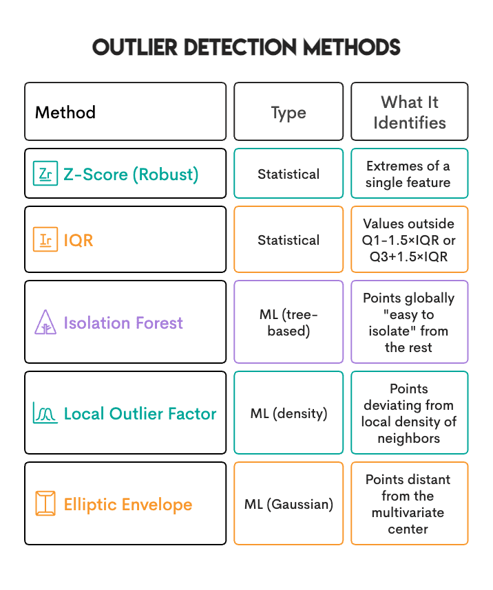
Here are the five methods we tested:
# First surprising discovery: Exaggerated results from multiple tests
Before comparing methods, I hit a wall. With 11 features, a naive approach (flag samples based on the extreme value of at least one feature) produced extremely inflated results.
IQR flagged approximately 23% of the wines as outliers. The Z-score flagged at about 26%.
If almost 1 in 4 wines is flagged as an outlier, something is wrong. There are no 25% outliers in the real dataset. The problem is that we are testing 11 features individually, which inflates the results.
The calculation is easy. With 11 independent features, if each feature has less than a 5% chance of having a “random” extreme value, we get:
\[ P(\text{at least one extreme}) = 1 – (0.95)^{11} \approx 43\% \]
Simply put, even if all the features were perfectly normal, we would expect that almost half of the samples would just happen to have at least one extreme value somewhere.
To fix this, I changed the requirements. Flag samples only if at least two features are extreme at the same time.

Changing min_features from 1 to 2 changed the definition from “The sample is extreme on any feature” to “The sample is extreme across multiple features.”
The code fix is as follows:
# Count extreme features per sample
outlier_counts = (np.abs(z_scores) > 3.5).sum(axis=1)
outliers = outlier_counts >= 2
# Comparison of five methods on one dataset
We counted the number of samples flagged by each method after the multiple testing fix was applied.

Here’s how to set up your ML method:
from sklearn.ensemble import IsolationForest
from sklearn.neighbors import LocalOutlierFactor

iforest = IsolationForest(contamination=0.05, random_state=42)
lof = LocalOutlierFactor(n_neighbors=20, contamination=0.05)
Why do all ML methods show exactly 5%? Because of contamination parameters. You want to flag exactly that percentage. It’s a quota, not a threshold. In other words, Isolation Forest flags 5%, regardless of whether your data contains 1% or 20% true outliers.
# Discover the real differences: identify what’s different
Here’s what surprised us the most. When examining how well the methods matched, Jaccard similarity scores ranged from 0.10 to 0.30. That’s a bad agreement.
Of 6,497 wines:
- Only 32 samples (0.5%) were flagged by all four major methods
- 143 samples (2.2%) were flagged in three or more ways
- The remaining “outliers” were flagged in only one or two ways
You might think it’s a bug, but that’s the point. Each method has its own definition of “abnormal”.

If a wine’s residual sugar level is significantly higher than the average, it becomes a univariate outlier (detected by Z-score/IQR). However, if you are surrounded by other wines with similar sugar content, LOF will not flag it. That’s normal in local situations.
So the real question is not, “Which method is best?” It’s “What kind of unusual thing am I looking for?”
# Health check: Do outliers correlate with wine quality?
The dataset contains expert quality ratings (3-9). We wanted to know: Do the detected outliers appear more frequently among wines with extreme quality ratings?
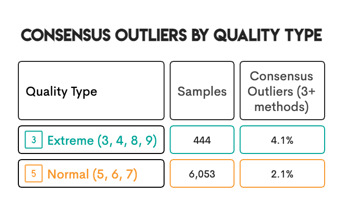
Extremely high-quality wines were twice as likely to be consensus outliers. That’s a good sanity check. In some cases, the relationship is obvious. Wines with too much volatile acidity taste like vinegar and are rated low and marked as outliers. A chemical reaction produces both results. However, we cannot assume that this explains all cases. There may be patterns we don’t see or confounding factors we don’t account for.
# Three decisions that shaped the outcome
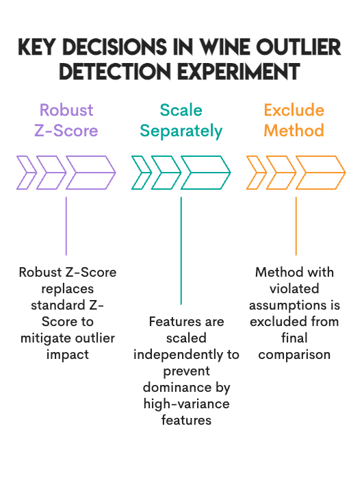
// 1. Use robust Z-scores instead of standard Z-scores
Standard Z-scores use the mean and standard deviation of the data, both of which are affected by outliers present within the dataset. Robust Z-scores instead use the median and median absolute deviation (MAD), both of which are not sensitive to outliers.
As a result, the standard Z-score identified 0.8% of the data as outliers, while the robust Z-score identified 3.5%.
# Robust Z-Score using median and MAD
median = np.median(data, axis=0)
mad = np.median(np.abs(data - median), axis=0)
robust_z = 0.6745 * (data - median) / mad
// 2. Scale red and white wine separately
Red wine and white wine have different standard levels of chemicals. For example, if you combine red and white wines into a single dataset, a red wine with perfectly average chemistry compared to other red wines may be identified as an outlier based solely on its sulfur content compared to the combined average of red and white wines. Therefore, we scaled each wine type separately using the median and interquartile range (IQR) for each wine type, and then combined the two.
# Scale each wine type separately
from sklearn.preprocessing import RobustScaler
scaled_parts = []
for wine_type in ['red', 'white']:
    subset = df[df['type'] == wine_type][features]
    scaled_parts.append(RobustScaler().fit_transform(subset))
// 3. Know when to exclude methods
Elliptical envelopes assume that the data follow a multivariate normal distribution. Ours wasn’t like that. The skewness of 6 of the 11 features exceeded 1, and 1 feature reached 5.4. I included the elliptical envelope in the comparison for completeness, but excluded it from the consensus vote.
# Determine which method performs best on this wine dataset
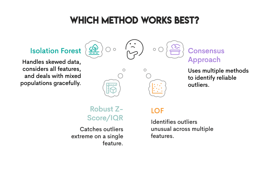
Image by author
Can we choose a “winner” given the characteristics of the data (high skewness, mixed population, unknown ground truth)?
Robust Z-scores, IQR, Isolation Forests, and LOF all handle skewed data well. If you have to choose one, choose Isolation Forest. It makes no distributional assumptions, considers all features at once, and handles mixed populations well.
But no single method can do it all.
- Isolation Forest may miss extreme outliers in only one feature (Z-score/IQR will detect them).
- Z-score/IQR can miss unusual outliers across multiple features (multidimensional outliers).
A better approach: Use multiple methods and trust consensus. The 143 wines flagged by three or more methods are much more reliable than those flagged by only a single method.
Here’s how consensus is calculated:
# Count how many methods flagged each sample
consensus = zscore_out + iqr_out + iforest_out + lof_out
high_confidence = df[consensus >= 3]  # Identified by 3+ methods
In the absence of ground truth (as in most real-world projects), method agreement is the closest measure of reliability.
# Understand what this means for your project
Define your problem before choosing a method. What is the “extraordinary” you are actually looking for? Data entry errors look different from measurement anomalies, and both look different from true rare cases. Different methods are presented depending on the type of problem.
Check your assumptions. If your data is highly skewed, standard Z-scores and elliptical envelopes can lead you in the wrong direction. Please check your distribution before committing to a method.
Use multiple methods. Samples flagged in three or more ways with different definitions of “outlier” are more reliable than samples flagged in only one.
Don’t think you need to remove all outliers. Outliers may be errors. It might also be the most interesting data point. Domain knowledge, not algorithms, makes the call.
# conclusion
The point here is not that outlier detection isn’t working. The meaning of “outlier” varies depending on who you ask. Z-score and IQR detect extreme values in a single dimension. Isolation Forest and LOF find samples that stand out within the overall pattern. Elliptical envelopes work well if your data is actually Gaussian (which ours was not).
Understand what you’re really looking for before choosing a method. Not sure? Try multiple methods and follow the consensus.
# FAQ
// 1. Decide which technique to start with
A good place to start is with the Isolation Forest technique. There is no expectation of how the data will be distributed or that all features will be used at the same time. However, if you want to identify the extremes of a particular measurement (such as a very high blood pressure reading), Z-scores or IQR may be a better choice.
// 2. Choosing contamination rates for Scikit-learn methods
It depends on the problem you’re trying to solve. A commonly used value is 5% (or 0.05). However, please note that pollution is a quota. This means that 5% of the sample will be classified as outliers, regardless of whether there are actually 1% or 20% true outliers in the data. Use contamination rates based on your knowledge of the proportion of outliers in your data.
// 3. Remove outliers before splitting training/testing data
no. You need to fit an outlier detection model to the training dataset and then apply the trained model to the test dataset. Otherwise, the test data will affect the preprocessing and cause leakage.
// 4. Processing categorical features
The techniques described here process numerical data. There are three possible alternatives for categorical features.
- Continue by encoding the categorical variable.
- Use techniques designed for mixed-type data (such as HBOS).
- Perform outlier detection separately for numeric columns and use frequency-based methods for categorical columns.
// 5. Know if a flagged outlier is an error or just an anomaly
Algorithms alone cannot determine when an identified outlier represents an error or is simply an anomaly. It doesn’t tell you what’s wrong, it shows you what’s abnormal. For example, a wine with a very high residual sugar content could be a data entry error. Or it could be a dessert wine meant to be that sweet. Ultimately, only domain expertise can provide the answer. If you’re unsure, mark it for review instead of automatically deleting it.
Nate Rossidi I am a data scientist and work in product strategy. He is also an adjunct professor of analytics and the founder of StrataScratch, a platform that helps data scientists prepare for interviews by providing real interview questions from top companies. Nate writes about the latest trends in the career market, offers interview advice, shares data science projects, and covers all things SQL.

