Human metabolome and machine learning improve prediction of post-mortem interval

Statistics and reproducibility

This study was approved by the Swedish Ethical Review Authority (Dnr 2019-04530 and Dnr 2025-0249-02). Due to the retrospective nature of the study, the Swedish Ethical Review Authority waived the need for informed consent. All methods were performed in accordance with relevant guidelines and regulations, and all samples were irreversibly anonymized before analysis. Autopsy cases were obtained from the Swedish National Forensic Board. After being transported to the autopsy site, the body is stored in a controlled indoor environment, typically a morgue’s refrigeration unit, which greatly reduces variation in decomposition rates compared to outdoor or uncontrolled conditions. See Supplementary Method 1 for details.

The original study included all autopsy cases admitted between September 1, 2017 and March 14, 2019. For independent testing data, cases were collected from January 1, 2021 to December 31, 2021. Inclusion criteria were: availability of femoral blood, age ≥18 years, and completion of toxicological screening using high-resolution mass spectrometry. See Supplementary Methods 1 for experimental details. No statistical methods were used to predetermine the sample size. No data were excluded from the analysis. The experiment was not randomized. The researchers were blinded to the assignments during the experiment and evaluation of results.

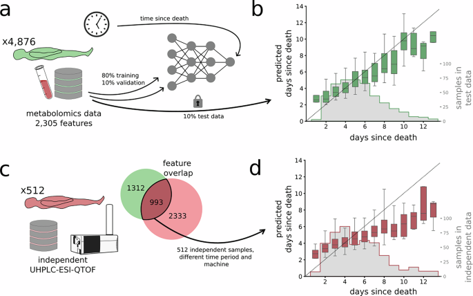
All autopsy cases from the original study period (September 1, 2017 to March 14, 2019) with a specific date of death or likely date of death (described below) were included (4876 autopsy cases in total). The most frequent causes of death in the study population, each with more than 100 cases recorded, included cardiovascular disease complications (n = 748), acute intoxication by one or more drugs (n = 659), hanging (n = 572), alcohol intoxication (221), drowning (194), multiple internal trauma injuries (150), and gunshot wounds (119). The demographic characteristics of the selected cohort can be summarized as follows. Age, median = 56 years (interquartile range = 39–69). Gender, male = 3544 (72.3%). BMI, median = 25.7 (interquartile range = 22.5–29.6). PMI, median = 5 days (interquartile range 4-7).

For independent laboratory data (January 1, 2021 and December 31, 2021), we randomly selected 512 autopsy cases with specific or estimated death dates (described below).

Calculation of post-mortem interval

In the database of the Swedish National Forensic Board, the date of death is estimated and coded in two different ways: certain and uncertain. For uncertain cases, the estimated date of death is given along with the date the deceased was last seen alive. This study includes all cases for which the date of death is certain (n= 3954). In addition, cases where the estimated date of death is included if the date of last seen alive was the day before the body was discovered (n= 922). This approach could include cases where, for example, a person was last seen alive in the evening and was found dead the next morning. However, there is also uncertainty of up to 48 hours in extreme cases (body was last found at 00:01 on day 1, body was found at 23:59 on day 2).

In some cases, the date of death was considered probable even if the date of last seen alive was the same date as the date of death. In Swedish forensic medicine, this is sometimes done to indicate that the death was not witnessed (i.e. the person was last seen alive in the morning and was found dead in the evening).

In this study, PMI is defined as the time (in days) between the date of death, definite or probable, as described above, and the date of autopsy when sampling was performed. In Sweden, autopsies are usually performed during morning work hours. So, for example, PMI = 2 can represent between 32 hours (body found and found on day 1 at 23:59, autopsy on the morning of day 3) and 80 hours (body found on day 2, last found at 00:01 on day 1, autopsy on the morning of day 4) for a case with a probable date of death.

Software implementation

Postmortem metabolomics data from the samples were preprocessed in R using the xcms and CAMERA packages as in ref. ³³. This workflow included peak detection, retention time alignment, feature grouping, and gap filling using the XCMS fillPeaks algorithm, resulting in 2305 metabolomic features. Missing values occurred when no metabolite peak was detected in a particular sample during XCMS processing. These missing peak intensities were substituted as zero values, reflecting metabolite abundance below the detection limit.

Computational analysis was performed in Python v. 3.12.4, relying primarily on the following packages: Keras v. 3.3.3, scikit-learn v. 1.5.0, numpy v. 1.26.4, scipy v. 1.13.1, matplotlib v. 3.8.4, and seaborn v. 0.13.2.

data processing

Data were normalized using logarithmic transformation (Equation 1).

$${x}_{norm}={{\rm{ln}}}(x+1)$$

(1)

where ×is the peak intensity, ×_nahrmeters This is a logarithmically transformed expression. Logarithmic transformation was applied to stabilize variance and reduce skewness, thereby reducing the heteroscedasticity inherent in the raw data. After log transformation, values for each metabolite were standardized using z-transformation (subtracting the mean of each log-transformed metabolic profile and dividing by the standard deviation). This step ensures that all metabolites are centered at zero and scaled to unit variance, facilitating comparisons between variables in downstream machine learning models. Logarithmic and Z-transformations addressed different aspects of the data distribution. The former reduced skewness and heteroscedasticity, and the latter ensured comparability of variables by placing them on a common scale. Exploratory analysis of the metadata suggested that batch effects and other sample-to-sample variations were minimal, so no additional corrections were applied.

We normalized and standardized the dataset before splitting it. Due to the large sample size, the difference in distribution between the full dataset and the training subset is expected to be minimal, and the impact on model performance is expected to be negligible. We used probabilistic assignment to randomly split the dataset into training (80%), validation (10%), and testing (10%).

Data harmonization between different datasets

To reconcile the variables of the independent test data with those of the original mass spectrometry dataset, we used a peak mapping approach to align features between the original and new datasets. Therefore, each feature in the original dataset defined by median mass-to-charge ratio (m/z) and retention time (RT) was matched with candidate features in the new dataset that were within the corresponding m/z and RT ranges. Among these candidates, the feature with the least squares distance from the m/z and RT of the original feature was selected as the best match. If there were no such candidates, the feature was set to 0. This mapping allowed us to sort the new dataset to match the feature structure expected by the model.

Neural network design and training

To predict PMI, we implemented a feedforward neural network regression model using the Keras package. To determine the optimal design of the model, we initiated hyperparameter optimization to select the number of hidden layers, the number of hidden nodes in each layer, and the dropout rate for each layer. Additionally, we implemented the option to train the model using a custom attention layer as an input layer, such that each metabolite is passed individually to a single node. The rationale behind this was that such an attention layer acts as a data-driven feature selection algorithm.

We trained each hyperparameter setting three times and selected the best performance using an early stopping algorithm with 25 epochs of patience in terms of prediction error on validation data. An early stopping algorithm was also used to restore the optimal weights during training. All tested hyperparameter sets can be found in Supplementary Data 5.

Training alternative machine learning models

We trained an alternative machine learning regression model using the same training data as the FFNN model. These models included two linear regression models: Ridge and LASSO. L₂ and L₁ Penalty weights were selected using Scikit-Learn’s built-in RidgeCV and LassoCV implementations. We also implemented gradient boosting and random forest regression models following the default settings of the Scikit-Learn package in Python. The default 100 estimators are used for each. Additionally, we also implemented K-nearest neighbor (K-NN) regression analysis and support vector regression (SVR) as implemented in Scikit-Learn. We trained the model using the assigned training data and tested it on the test data to ensure consistency. The settings used in the alternative machine learning method can be found in Supplementary Data 5.

Extraction of learned model structure and identification of features

We sought to extract which metabolomic features are used in the decision-making process of each model. Extracting such input-output dependencies is not easy for neural networks;^34,35We used the attention layer of FFNN to estimate the usage of input variables. By analyzing the activation of these input nodes and correlating them with the PMI, we generated a list of metabolomic features ranked by importance.

All metabolomic features included in the FFNN were uploaded to MetaboAnalyst (version 6.0) for functional analysis. This is suitable for untargeted metabolomics data based on the assumption that putative annotations at the compound level can collectively predict functional changes at the group level defined by a set of metabolite pathways.³⁶.

Metabolomic features important for decision-making in FFNN were identified and annotated putatively by reviewing compound hits from functional analysis in MetaboAnalyst and/or by matching mass-to-charge ratio (m/z; ± 5 ppm) to the online human metabolome database (HMDB; https://hmdb.ca).