Framework and workflow
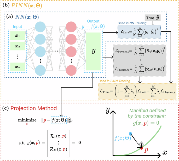
A schematic workflow of our approach is illustrated in Fig. 1. Both systems under study are described by a set of coupled ODEs, and their numerical solution is used as the ground truth. We then train two models: an artificial NN data-driven model (Fig. 1a), and a model where the physics priors are included in the loss function, hereafter denoted as loss-based PINN (Fig. 1b). Specifically, our method is applied as follows: (i) one input vector in provided to the already trained NN model and a prediction vector f (x; Θ) is obtained; (ii) p is initilized with the output vector f (x; Θ); (iii) the constrained optimization problem is solved by Eq. (1) and the result of the optimization is the corrected output vector p. This way, p is a point that lies on the physical manifold and thus, by enforcing the physics constraint post-training at inference time, we guarantee that the final prediction is physics-consistent (Fig. 1c). Figure 1c also makes clear the intuition behind the projection method. The same process is applied to each point prediction of the loss-based PINN.

a Artificial NN data-driven model y = f(x; Θ), where x represents the input vector, y is the predicted output vector, and Θ denotes the model parameter vector. b Loss-based PINN model with a regularization term in the loss function, where \({\hat{{{\bf{y}}}}}_{{{\bf{i}}}}\) represents the target output vector, yi represents the predicted output vector, \({{{\mathcal{L}}}}_{{\rm {Data}}}\) represents the data loss term between the PINN’s predicted outputs and the target data, \({{{\mathcal{R}}}}_{j}\) represents the residual associated with the jth physical law, \({{{\mathcal{L}}}}_{{\rm {Physics}},j}\) represents the physics loss term regarding the jth physical law imposed to the system, \({{{\mathcal{L}}}}_{{\rm {Train}}}\) represents the total training loss function, which is a weighted sum balancing data fitting and adherence to physical constraints, and λj represents the weight factor given to the jth physical law, with \(\lambda ={\sum }_{j = 1}^{M}{\lambda }_{j}\le 1\). c Formulation and visualization of the projection operation method as a constraint optimization problem, with the projection of the output y of the model onto the manifold defined by the constraint vector g(x, y) = 0, where W is a symmetric positive weight matrix.
The NN and the loss-based PINN models are used here as base models to demonstrate the proposed projection method. Note, however, that our approach is model-agnostic and can be applied to the predictions of any ML model (e.g., support vector regression or linear regression), as it requires only the physical laws, defined by g(x, p), and a point prediction from the base model, denoted by f (x; Θ). Moreover, it is worth emphasizing that our loss-based PINN, where the physical constraints are very general physical principles, corresponds to problems where the physics laws are more general than in the usual application of PINNs and where PINNs have seldom been tested.
Our analysis focuses on comparing the accuracy of the results before and after the projection of the models’ predictions. Additionally, we analyze the robustness of our method across varying model complexity and training, and discuss the physical insight into the underlying physics.
Case study 1: spring-mass system
This example highlights the ability of the projection method to handle sequential predictions and how it corrects the trajectories as they gradually deviate from the target values.
System description
The system consists of two masses, m1 and m2, connected in series by two springs with spring constants k1 and k2, and natural lengths L1 and L2, respectively. The first spring is connected to a fixed wall at one end and to mass m1 at the other, while the second spring connects the two masses. The masses are restricted to moving along the x-axis, and there is no friction. The positions of m1 and m2 along the x-axis are denoted by x1 and x2, and their velocities by v1 and v2, respectively. The forces exerted by the springs on the masses are determined by the displacements from their equilibrium positions, following Hooke’s law.
The differential equations of motion are given by
$$\left\{\begin{array}{l}{m}_{1}{\ddot{x}}_{1}=-{k}_{1}({x}_{1}-{L}_{1})+{k}_{2}({x}_{2}-{x}_{1}-{L}_{2})\quad \\ {m}_{2}{\ddot{x}}_{2}=-{k}_{2}({x}_{2}-{x}_{1}-{L}_{2})\quad \hfill\end{array}\right.,$$
(2)
where \({\ddot{x}}_{1}\) and \({\ddot{x}}_{2}\) denote the accelerations of masses m1 and m2. The time-evolution of the system is determined from the solution of these equations, with the initial conditions
$$\left\{\begin{array}{l}{x}_{1}(0)={x}_{0,1},\quad {x}_{2}(0)={x}_{0,2}\quad \\ {v}_{1}(0)={v}_{0,1},\quad {v}_{2}(0)={v}_{0,2}\quad \end{array}\right..$$
(3)
Since there is no friction, the mechanical energy, E, defined by the sum of the kinetic energy of the masses and the elastic potential energy, is conserved. Hereafter we consider m1 = 1 kg, m2 = 1 kg, k1 = 5 N m−1, k2 = 2 N m−1, L1 = 0.5 m, and L2 = 0.5 m.
Data generation
The artificial NN data-driven model takes as input a state vector characterizing the state of the system at the current instant t (i.e., defining the positions and velocities of both masses at time t), and predicts the state vector at time t + Δt, for fixed Δt. This procedure enables the recursive determination of the complete trajectory from a given initial condition, with time-resolution Δt = 50 ms, as a sequence of transitions between states. We used an energy threshold \({E}_{\max }=\) 5 J to create a set of allowed states for the system, corresponding to the range of positions and velocities the masses can have with E < Emax. Eq. (2) was solved using the classical fourth-order Runge–Kutta method (RK4), with arbitrary initial conditions (3) ensuring that \(E < {E}_{\max }\).
Except otherwise noted, the dataset consists of N = 100,000 arbitrarily generated input state vectors within the energy threshold and the corresponding next states, determined by performing a single Runge–Kutta computation up to time Δt (not to be confused with the Runge–Kutta time-step). To reduce the impact of the difference in feature magnitude on the model and make the training process more stable, we applied the min–max normalization. Consequently, all features were scaled to the range [−1, 1].
Trajectory prediction
The trajectory of the system is defined by the prediction of its state along 165 sequential time steps, i.e., 8.25 s. The general physical law considered in the loss-based PINN and in the projection method is energy conservation, which translates into the residual \({{{\mathcal{R}}}}_{1}=E
(4)
where asi and bsi are the stoichiometric coefficients of species s, as they appear on the left- and right-hand sides of a reaction i, respectively. In addition, the average gas temperature Tg and the gas temperature near the tube wall Tnw are calculated from the gas thermal balance equation, the reduced electric field E/N, where N is the gas density, from the quasi-neutrality condition, the electron drift velocity vd and temperature Te as integrals over the electron energy distribution function, and the electron density from the discharge current. Further details are given in ref. 25.
Data generation
The models include three input features (P, I, and R) and the 17 outputs just described. We generated the datasets with the LisbOn KInetics Chemistry+Boltzmann (LoKI-B+C) simulation tool25,26. Except otherwise noted, the dataset comprises N = 1000 uniformly distributed values across the three input features within their specified boundaries. Similarly to the previous case, we applied the min-max normalization to the features, scaling them to the range [−1, 1]. Moreover, we applied a log-transformation to the features demonstrating skewness in their distribution. Further details on data generation and preprocessing are given in the “Data pre-processing” subsection in the “Methods” section.
Prediction of the steady-state plasma properties
The general physical laws constraining the system include: the ideal gas law, relating the gas pressure (input) with the species densities and the gas temperature (outputs); the imposed discharge current (input), expressing electric charge conservation and relating its input value with the tube radius (input), and with the drift velocity and electron density (outputs); and the quasi-neutrality law, relating the electron density (output) with the positive and negative ion densities (outputs). These laws can be represented by the residuals in Eqs. (5)–(7), respectively,
$${{{\mathcal{R}}}}_{1}=P-{\sum}_{i}[{X}_{i}]{k}_{{\rm {B}}}{T}_{{\rm {g}}}$$
(5)
$${{{\mathcal{R}}}}_{2}=I-e{n}_{{\rm {e}}}{v}_{{\rm {d}}}\pi {R}^{2}$$
(6)
$${{{\mathcal{R}}}}_{3}={n}_{{\rm {e}}}-{\sum}_{i}[{X}_{i}^{+}]+{\sum}_{j}[{X}_{j}^{-}]$$
(7)
where [Xi] is the density of species i, ∑i[Xi] is the total gas density given by the sum of all the species densities, kB is the Boltzmann constant, e is the charge of the electron, \({\sum }_{i}[{X}_{i}^{+}]\) is the sum of the positively charged ion population, and \({\sum }_{j}[{X}_{j}^{-}]\) is the sum of the negatively charged ion population.
The test-set results of the four models on the prediction of the 17 output variables and on the three physical laws are shown in Fig. 4a, b, respectively, expressed as root mean squared errors (RMSE). Applying the projection method to NN predictions reduces the RMSE of compliance with physical laws by more than 9 orders of magnitude, while improving predictive accuracy of three of the output variables: O2(X), \({{{\rm{O}}}}_{2}^{+}\), and ne. As it was the case in the spring-mass system, imposing very general physical laws is ineffective in guiding the loss-based PINN model, which is not able to reduce the RMSE of compliance with physical laws (Fig. 4b) nor of the predicted outputs, when compared with the NN model.

a Test set results of the four models (NN (blue), loss-based PINN (pink), projected NN (red), and projected PINN (green)) when predicting the 17 outputs. The predicted outputs include 11 species densities (O2(X) and atoms O(3P), electronically excited states \({{{\rm{O}}}}_{2}(a{}^{1}{\Delta }_{g},b{}^{1}{\Sigma }_{g}^{+},{{\rm{Hz}}})\) and O(1D), ground-state ozone O3 and vibrationally excited ozone \({{{\rm{O}}}}_{3}^{\star }\), negative ions O−, and positive \({{{\rm{O}}}}_{2}^{+}\) and O+ ions), the average gas temperature Tg and the gas temperature near the tube wall Tnw, the reduced electric field E/N, where N is the gas density, the electron drift velocity vd and temperature Te, and the electron density ne. b Test set results of the four models when evaluating the compliance with physical laws (the ideal gas law (pink), electric charge conservation (green), and the quasi-neutrality law (yellow)). c Relative density of the main species in the mixture at steady-state. d Bar plot of the three outputs that improved the most when the projection method was applied to the NN predictions. For each output is presented the RMSE of the NN (blue), the projection when the three constraints are applied simultaneously (red), the projection when the constraints are applied individually (pink, green, yellow), and the projection when the constraints are applied in pairs (brown, purple, cyan). `P constraint’ refers to the ideal gas law, `I constraint’ refers to the electric charge conservation, and `Neut. constraint’ refers to the quasi-neutrality law.
Figure 4c, d provides insight into the physical interpretation of the results, by representing the main species in the mixture and examining the effects of each physical constraint individually. Ground-state O2(X) molecules constitute 88.3% of the total mixture, and the prediction of their density improves primarily due to the ideal gas law constraint (5), which explicitly accounts for species densities. Similarly, the electron density ne benefits from the imposition of the discharge current constraint (6), as it appears directly in the expression of this law. Finally, \({{{\rm{O}}}}_{2}^{+}\) constitutes <0.0001% of the gas mixture and, as expected, remains unaffected by the ideal gas law (5). It is the dominant positive ion by at least 2 orders of magnitude25, making its prediction inherently sensitive to the quasi-neutrality condition (7). However, this constraint alone is insufficient to correct the prediction, as the electron density sets an “anchor” for the total ion density. Therefore, the accuracy of the \({{{\rm{O}}}}_{2}^{+}\) density in the projection method is coupled with the prediction of ne, and both the discharge current (6) and quasi-neutrality (7) laws are required to improve the model’s performance regarding this output.
Robustness of the projection method
With sufficient training time and a sufficiently complex architecture, a neural network can produce predictions that closely approximate the target values, reducing (or even eliminating) the need for post-training corrections. Conversely, a poorly trained model may yield predictions that deviate significantly from the manifold defined by the physical laws, making the projection operation ineffective or leading to ambiguities associated with multiple possible solutions. In this section, we analyze the robustness of the projection method with respect to model complexity, quantified by the number of NN parameters (i.e., weights and biases) and the size of the training dataset. The results focus on the low-temperature reactive plasma system described in the “Case study 2: low-temperature reactive plasma” subsection in the “Results and discussion” section.
Ablation study
We start by comparing the errors before and after applying the projection operation to the NN predictions, considering models with different complexities. In order to guarantee a comparable analysis between the models, we considered 18 different architectures, each with 2 hidden layers and a number of neurons ranging from 1 to 1000 in the hidden layers. Both hidden layers have the same number of neurons. For each architecture, 1 NN model was trained with a dataset consisting of N = 1000 data points.
Figure 5a.i shows the RMSE of the predictions of the NN and of the projection method as a function of the number of parameters in the model. These values are calculated by averaging the errors across the 17 outputs. The “RMSE variation rate” is defined as the relative change in RMSE after performing the projection and is considered negative if the RMSE decreases. Figure 5a.ii provides a similar analysis, but for the 3 outputs that improved the most after applying the projection operation, as opposed to the mean of all outputs. The graphs show that the NN projection consistently achieves lower RMSE than the standard NN. The improvement is particularly pronounced for O2(X), \({{{\rm{O}}}}_{2}^{+}\) and ne predictions, in simpler models with fewer parameters (~102). As the number of parameters increases to 105, both methods reach a performance plateau, and the advantage of the projection method becomes marginal, though it still yields slightly better predictions. These results suggest that the projection method is particularly beneficial for more constrained, and hence computationally more efficient, NN architectures.

a RMSE of the NN and the NN projection as a function of the model complexity (number of weights and biases in the NN architecture). Blue solid lines with circle markers represent the NN predictions, red dashed lines with circle markers represent the projected NN predictions. The green solid line with circle markers in (i) represents the error variation rate before and after applying the projection to the NN outputs. b NN and NN projection pressure related trends of the electron density, ne, for I = 30 mA, R = 12 mm, and the following NN architectures: (i) [8,8]; (ii) [26,26]; (iii) [1000,1000]. The target values (red crosses) are obtained from LisbOn KInetics (LoKI) simulation tool. Blue solid lines represent the NN predictions, green dashed lines represent the projected NN predictions.
It is instructive to analyze the predictions of pressure-dependent trends for fixed discharge current and tube radius. Figure 5b.i–iii illustrates how NN architectures of increasing complexity predict ne as a function of pressure for I = 30 mA and R = 12 mm, and benchmarks these predictions to LoKI simulation values. In the simplest architecture (Fig. 5b.i), the predictions of the NN deviate significantly from the targets in both magnitude and trend (RMSE = 2.55 × 10⁻²). Despite this poor initial performance, the projection successfully aligns the predictions with the LoKI targets (RMSE = 0.53 × 10⁻²), albeit with a visible lack of smoothness. In the intermediate case (Fig. 5b.ii), the projection method smooths the noisy NN curve, reducing the RMSE in ~57%. Finally, in the most complex architecture (Fig. 5b.iii), the NN starts to align with the target values, indicating that sufficient model complexity can compensate for the absence of explicit physical information, though at the cost of increased computational resources.
Small samples
We now compare the errors before and after applying the projection operation to the NN predictions, considering training datasets with different sizes. In order to guarantee a comparable analysis between the models, an architecture with 2 hidden layers and 50 neurons in each layer was used. To mitigate randomness associated with a specific dataset sample, 20 random samples are drawn for each dataset size from a larger dataset. The NN model is then trained on each sample, and the trained models are evaluated on a test set to obtain errors for each of the 17 outputs. The results are shown in Fig. 6a.i, where each point represents the mean error across the 20 samples for each dataset size, considering the average performance on the 17 output predictions. Furthermore, 11 different dataset sizes were analyzed, ranging from 20 to 2500 observations. The aggregate RMSE across all 17 output quantities decreases consistently as the dataset size grows, with both methods showing similar rates of improvement. The projection method maintains a persistent advantage of approximately −2.4% to −2.8% in RMSE variation rate compared with the NN.

a RMSE of the NN and the NN projection as a function of the dataset size. Blue solid lines with circle markers represent the NN predictions, red dashed lines with circle markers represent the projected NN predictions. The green solid line with circle markers in (i) represents the error variation rate before and after applying the projection to the NN outputs. b NN and NN projection pressure related trends of the electron density, ne, for I = 30 mA, R = 12 mm, and the following dataset sizes: (i) 200; (ii) 600; (iii) 2500. The target values (red crosses) are obtained from LisbOn KInetics (LoKI) simulation tool. Blue solid lines represent the NN predictions, green dashed lines represent the projected NN predictions.
Figure 6a.ii depicts a similar RMSE analysis as in Fig. 6a.i, but for the three most relevant individual outputs. A similar conclusion as in the previous section can be drawn: the projected predictions outperform the non-projected counterparts, particularly for smaller dataset sizes, where the model benefits the most from the addition of physical constraints. This is further confirmed by inspection of Fig. 6b, representing the predictions of the electron density as a function of pressure, for the same discharge current and tube radius as in Fig. 5b. With limited training data (Fig. 6b.i), the NN predicts a nonphysical behavior at higher pressures, with a sharp decrease above 800 Pa that contradicts the expected saturation pattern. In contrast, the projection method maintains physically sound predictions across the entire pressure range, effectively compensating for the scarce training data. As expected, the accuracy of the NN progressively improves when trained on larger datasets (Fig. 6b.ii, iii), while the projection method’s predictions remain more accurate and consistently aligned with physical expectations. These results demonstrate the role of the projection method as an efficient procedure to include physical constraints into the predictions in scenarios where scarce data is available, maintaining physically meaningful predictions and substantial error reductions with limited training samples.
Computation time
To evaluate the computational performance of our approach, we compare the total computation time required by both the NN and the NN projection methods. Figure 7a depicts the mean RMSE of the predictions for O2(X), \({{{\rm{O}}}}_{2}^{+}\), and ne as a function of the time required to train the models of varying complexity (described in the “Ablation study” subsection in the “Results and discussion” section) and to evaluate their predictions in a test set. For the NN projection method, the total computation time includes the NN training and inference times, as well as the additional time required to project the outputs onto the physically consistent manifold. The curves correspond to an exponential fitting function to the data and are merely a guide to the eye. We observe that models with longer training times benefit the most from the projection method. Moreover, on average, the projection step takes only 1.75 s for a dataset of 500 observations, which corresponds to a modest 4.33% increase in the total computation time when compared with the NN model. This slight increase in computation time of the projection method comes with a reduction of the RMSE by an average of 32.08%, with improvements reaching up to 63.86% in simpler architectures that require more epochs to converge.

a Analysis for models with ranging complexity. b Analysis for models trained with datasets of different sizes.
Figure 7b illustrates the mean RMSE of the predictions as a function of the total time required to generate data sets of different sizes (described in the “Small samples: subsection in the “Results and discussion” section), train the models, and evaluate their predictions in a test set. As expected, increasing the dataset size leads to lower RMSE values for both models, but at the cost of significantly longer computation times. Clearly, the NN projection is computationally more efficient than the purely data-driven NN, despite the additional projection step. As an example, the NN trained with 200 observations achieved an RMSE of 0.050, requiring a total computation time of 4913 s. In contrast, applying the projection method to the predictions of the NN trained with only 50 observations resulted in a comparable RMSE of 0.048, but with a significantly reduced computation time of 1338 s. This represents a reduction in computational cost by a factor of ~3.7 while maintaining a nearly identical predictive accuracy.