Theoretical framework
Our framework, which integrates neural network potential and polarizable long-range interactions, is depicted in Fig. 1. For a given chemical system and boundary conditions, our goal is to construct a mapping from atomic coordinates \({{{{\bf{r}}}}}_{i}\) and atomic types \({Z}_{i}\) to the total potential energy \({E}_{{{{\rm{pot}}}}}\). The potential energy is expressed as the sum of the second-order expansion30 with respect to charge fluctuations and the density functional theory39 D3 (DFT-D3) van der Waals dispersion energies correction term40,41 \({E}_{{{{\rm{D}}}}3}\),
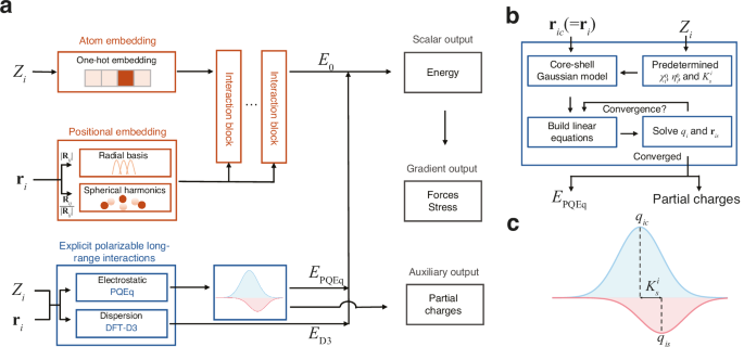
$${E}_{{{{\rm{pot}}}}} ={\sum }_{i}\left(\,{E}_{0}^{i}\left({{{{\bf{r}}}}}_{i},\,{Z}_{i}\right)+{\chi }_{i}^{0}{q}_{i}+\frac{1}{2}{\eta }_{i}^{0}{q}_{i}^{2}+\frac{1}{2}{K}_{s}^{i}{\left|{{{{\bf{r}}}}}_{{ic}}-{{{{\bf{r}}}}}_{{is}}\right|}^{2}\right)\\ \;\;\;+{\sum }_{{ik} > {jl}}{C}_{{ik},{jl}}\left({{{{\bf{r}}}}}_{{ik},{jl}}\right){q}_{{ik}}{q}_{{jl}}+{E}_{{{{\rm{D}}}}3}\\ ={\sum }_{i}{E}_{0}^{i}+{E}_{{{{\rm{PQEq}}}}}+{E}_{{{{\rm{D}}}}3}.$$
(1)

a The framework takes atomic numbers (\({Z}_{i}\)) and coordinates (\({{{{\bf{r}}}}}_{i}\)) as inputs and integrates a neural network block and an explicit polarizable long-range interactions block. For the neural network block, atomic numbers are converted into feature vectors via one-hot encoding, while the coordinates are transformed into a representation of the local environment using radial basis functions and spherical harmonics to capture the distance (\({|{{{\bf{R}}}}}_{{ij}}|\)) and directional (\({{{{\bf{R}}}}}_{{ij}}/|{{{{\bf{R}}}}}_{{ij}}|\)) information. These embeddings are processed through an equivariant graph neural network to output the scalar machine learning potential energy \({E}_{0}\). Explicit, physically-grounded calculations are performed for long-range effects. An electrostatic energy component (\({E}_{{{{\rm{PQEq}}}}}\)) is calculated using the polarizable charge equilibration (PQEq) method, and a dispersion energy component (\({E}_{{{{\rm{D}}}}3}\)) is calculated using the DFT-D3 method. The total energy is the sum of these components. Gradients of the energy yield forces and stress on the system. The long-range block also provides partial charges as an auxiliary output. b A flowchart detailing the iterative self-consistent procedure for the PQEq method. Starting with atomic core positions (\({{{{\bf{r}}}}}_{{ic}}\)), atomic numbers (\({Z}_{i}\)), and predetermined atomic parameters (electronegativities \({\chi }_{i}^{0}\), chemical hardness \({\eta }_{i}^{0}\), and spring constant \({K}_{s}^{i}\)), the method uses a core-shell Gaussian model to build and solve a system of linear equations. This loop is repeated until the partial charges (\({q}_{i}\)) and shell positions (\({{{{\bf{r}}}}}_{{is}}\)) converge, yielding the final electrostatic energy (\({E}_{{{{\rm{PQEq}}}}}\)) and the converged partial charges. c Partition of core-shell Gaussian charge model used in long-range electrostatics. The partial charge (\({q}_{i}\)) of each atom is represented as the sum of the core (\({q}_{{ic}}\)) and shell (\({q}_{{is}}\)) charge. The harmonic spring constant, \({K}_{s}^{i}\), couples the core and shell.
The zeroth-order atomic energy \({E}_{0}^{i}\) corresponds to the final layer scalar output of the equivariant graph neural networks, while the higher-order self- and interatomic Coulomb interactions represent the polarizable long-range electrostatic interactions \({E}_{{{{\rm{PQEq}}}}}\). To account for charge transfer and polarization effects, the partial atomic charge \({q}_{i}\) of atom i is the sum of the nuclear core charge \({q}_{{ic}}\) and shell charge \({q}_{{is}}\), both of which assume a Gaussian charge distribution form. The first-order coefficients \({\chi }^{0}\) are electronegativities, commonly defined as half of the sum of ionization potential (IP) and electron affinities (EA). The second-order coefficients \({\eta }^{0}\) signifies idempotential or chemical hardness, defined as \({{{\rm{IP}}}}-{{{\rm{EA}}}}\). The spring constant \({K}_{s}^{i}\) denotes the isotropic harmonic connectivity between the shell position \({{{{\bf{r}}}}}_{{is}}\) and core position \({{{{\bf{r}}}}}_{{ic}}\) (equal to \({{{{\bf{r}}}}}_{i}\)) of atom i. The Gaussian electrostatic energy is given by \(C\left({{{{\bf{r}}}}}_{{ik},{jl}}\right){q}_{{ik}}{q}_{{jl}}\), where i and j are the atomic indices, and k and l represent the core (c) or shell (s), respectively. The displacement vector is given by \({{{{\bf{r}}}}}_{{ik},{jl}}={{{{\bf{r}}}}}_{{ik}}-{{{{\bf{r}}}}}_{{jl}}\). The detailed derivation of the response to the external electric field can be found in the Supplementary Note 1. In previous works, PQEq parameters for 102 elements have been derived from experimental data or high-level QM calculations25,42, and have accurately reproduced QM electrostatic interaction energies30. In the equivariant neural networks12, the initial features are generated using a trainable one-hot embedding that operates on the atomic types. The interatomic distance of atom i and atom j, denoted as \(|{{{{\bf{R}}}}}_{{ij}}|\), is expanded by radial basis functions. Concurrently, the directional component of the interatomic vectors, expressed as \({{{{\bf{R}}}}}_{{ij}}/|{{{{\bf{R}}}}}_{{ij}}|\), is expanded by spherical harmonics functions. These features are utilized to construct the atomic graph. Then, through the equivariant message passing23 schemes, the atomic features are updated. A multilayer perceptron layer is then connected to derive the scalar output. It should be noted that the neural network potential component is specifically designed to capture energy contributions distinct from electrostatic interactions, thereby ensuring no overlap in energy accounting between different components. Subject to the conservation of the net charge and the equality of chemical potentials for all atoms, the linear equations can be used to update partial charges (\({q}_{i}\)) and shell positions (\({{{{\bf{r}}}}}_{{is}}\)). The partial charges can be obtained self-consistently in each MD step. The forces on atoms and virial stress on the cell can be calculated via automatic differentiation after partial charges are determined, as detailed in Supplementary Note 2.
Validation on diverse charge-state datasets
To evaluate the capability of our framework in capturing different charge states and long-range interactions, we validated our framework against the dataset developed by Ko et al.28 and Maruf et al.38, which encompass various charge states and charge transfer systems. They contain six distinct subsets: Ag cluster with positive and negative total charge, (Ag3+/−), Na-Cl ionic cluster with one neutral Na removed (Na8/9Cl8+), hydrogenated carbon chains in both neutral and cationic states (C10H2/C10H3+), a periodic system consisting of Au clusters adsorbed on an MgO-(001) surface, and benzotriazole interactions with Cu-(111) surfaces in dry (BTA-Cu) and aqueous (BTA (H2O)-Cu) environments. We demonstrate the advantage of integrating equivariant message-passing networks with explicitly polarizable long-range interaction models by benchmarking against both 4G-HDNNP, a local MLIP with explicit long-range interactions, and NequIP, which implicitly captures long-range effects through its message-passing mechanism. 4G-HDNNP differentiates charged systems by explicitly training DFT partial charges and incorporating them as descriptors into neural networks for short-range interactions. We employed the NequIP models trained in the reference38 (Maruf’s NequIP) as our baseline equivariant model. Our framework explicitly incorporates long-range interactions while adopts Maruf’s NequIP as the E0 component without touching its settings, thereby ensuring a fair comparative analysis. The results are presented in Table 1, with detailed neural network architectural specifications provided in the Supplementary Table 3.
For the carbon chains, the introduction of additional H+ causes some C atoms to exhibit opposite charge states43, as shown in Supplementary Fig. 1a. Although we did not fit partial charges, our model qualitatively captures the distribution of DFT partial charges, as shown also in Supplementary Fig. 1a. In the linear C10H2 molecule, our model demonstrates symmetric charge distribution around the center which shows agreement with DFT. After explicitly incorporating physical long-range interactions, our framework achieved additional improvements in error metrics compared to NequIP and 4G-HDNNP. For positively charged NaCl clusters, the predicted energy and forces by our model are still more accurate compared to 4G-HDNNP, as well as the potential energy surface shown in Supplementary Fig. 1b. For Au2 adsorption on MgO surfaces and benzotriazole interactions with Cu-(111) surfaces in dry and aqueous environments, our model outperforms NequIP significantly. Additionally, our model correctly predicted the preferential adsorption geometries for both doped and undoped MgO, as listed in Supplementary Table 1. As for the charged Ag clusters, due to their small system size and lacking long-range effects, the entire structure falls within the typical cutoff radius used by the MLIP. The energy dependence on the overall charge state of clusters leads to degeneracy between atomic structures and potential energy surfaces, resulting in poor performance of the charge-independent NequIP model. We acknowledge that for such small, highly charged systems, the 4G-HDNNP approach to learning charge equilibration parameters is more convenient. Nonetheless, we also achieved reduced force error with the fixed physical parameters compared to 4G-HDNNP. Although PQEq partial charges are not directly comparable to DFT Hirshfeld ones, we compare them to show their relevance. Varying degrees of agreement across different chemical systems are observed, as shown in Supplementary Table 2.
Our comprehensive evaluation demonstrates that explicit incorporation of physical long-range interactions significantly enhances the performance of MLIPs across diverse charge-state systems. Notably, our proposed framework outperforms 4G-HDNNP in most cases for energies and forces without fitting partial charges. This advantage likely stems from a more physically meaningful partition of the total energy.
Foundation model benchmark
We trained a foundation model for all the periodic table elements up to Pu using the MPtrj dataset16 following our framework (our model), as described in the Methods section. We also trained a model maintaining the same MLIPs framework and dataset, but without the polarizable long-range interactions (w/o-lr model). The former one demonstrated mean absolute errors (MAE) of 18 meV per atom for energies, 0.065 eV\(\cdot\)Å−1 for forces, and 0.301 GPa for stresses across the test set, outperforming the w/o-lr model, as shown in Supplementary Table 4. These proved the benefit of incorporating long-range interactions in the enhancement of prediction accuracy.
Message-passing mechanisms will fail when graph connections break in the system. For instance, in dimers, when the interatomic distance exceeds the graph cut-off, the atoms no longer interact with each other. We analysed interaction energies for Na-Na and Na-Cl dimers across interatomic distances ranging from 1.8 Å to 12.0 Å. As shown in Fig. 2a, both models (our model and the w/o-lr model) trained on the MPtrj dataset accurately reproduce the equilibrium bond lengths of the two dimers. However, the w/o-lr model failed to differentiate interaction energies beyond the MLIPs cutoff distance, i.e., 5.0 Å, while our model successfully captured the DFT potential energy surface throughout the entire distance range, demonstrating its capability in describing extended ionic interactions. Moreover, the message-passing mechanism exhibits deficiencies when simulating layered materials. Taking lithium iron phosphate (LiFePO4) as a case study, we observed that the w/o-lr model predicted an irreversible phase transition, as shown in Supplementary Fig. 3. In contrast, our model correctly reproduced the experimentally44 and AIMD45 thermally stable olivine structure. These results collectively demonstrate that the explicit long-range interactions are crucial for accurately describing both ionic systems and layered materials, particularly in predicting structural stability and thermal behavior.

a The interaction energies for Na-Na (green) and Na-Cl (purple) dimers predicted by our model, the model without polarizable long-range interactions (w/o-lr model), and reference calculations using density functional theory (DFT)39. b Evaluation of polarizable interactions in water molecules. The water molecule model is oriented in the yz-plane, with oxygen and hydrogen atoms shown in red and white, respectively. The energy response curves as a function of external electric field (\({{{\mathbf{\epsilon }}}}\)) strength applied along the x-axis. Results are compared among our model (red), the Charge Equilibration (QEq)-based model25 (blue), and the reference DFT calculations (gray) serving as the reference values. c–e Comparison of bulk modulus from DFT calculations (reference values) and our model (prediction values): (c) Voigt approach (BV), (d) Reuss method (BR), and (e) Hill average (BVRH). The R-squared values (R2) and mean absolute errors (MAE) of the bulk modulus are also shown.
Polarization plays a fundamental role in determining molecular responses to external electric fields. Conventional QEq-based models have limitations in their response to an external electric field applied orthogonally to the molecular dipole. We validated this capability through a benchmark study examining a water molecule’s response to external electrostatic fields46. The water molecule was fixed in the yz-plane, and we applied varying external electric fields along the x-axis to derive energy curves, with the results presented in Fig. 2b. The model with polarizable long-range interactions demonstrates a trend consistent with the reference values obtained from DFT. Due to the external electrostatic field direction consistently being orthogonal to the molecule, the electrostatic energy in the QEq-based model (like 4G-HDNNP) is 0 and is completely independent of field strength (i.e., \({{{\mathbf{\mu }}}} \, {{\cdot }} \, {{{\mathbf{\epsilon }}}}=0\), where \({{{\mathbf{\mu }}}}\), \({{{\mathbf{\epsilon }}}}\) are dipole moment and electric field, respectively). This is because the QEq model treats atoms in the molecule as point charges or Gaussian charges, without distinguishing between core and shell components. We also compared the response of O atom partial charges across DFT Hirshfeld calculations, our model, and the conventional QEq model, as shown in Supplementary Fig. 4. The agreement between the PQEq model and DFT is observed, while the QEq model completely lacks response. This comparative analysis establishes that the explicit polarizable interactions are crucial for modeling molecular systems subject to external electric fields.
Besides the failure of response in static conditions, the QEq method may exhibit non-physical behavior in dynamics47. As illustrated in Supplementary Fig. 5, we conducted additional investigations of two water molecules under an external electric field of 0.25 V\(\cdot\)Å−1. In charge distribution models, it is essential to allow systems to form an internal electric field opposing the external field. The QEq model assumes the system behaves as a perfect conductor without penalizing charge transfer as a function of distance. This limitation of the QEq method leads to non-physical charge transfer between molecules separated by large distances47. In contrast, within the PQEq model, the individual water molecules can polarize, generating internal electric fields that counteract the external field, thereby capturing more realistic electrostatic responses in molecular systems. Under the QEq scheme, the water molecules accumulate non-zero net charges and migrate to the top and bottom of the simulation box. In contrast, our model maintains charge neutrality of the water molecules, which remain stationary despite the applied electric field, aligning with DFT results.
We conducted benchmarking using properties that were not labeled during the training process. We applied our foundation model to predict the mechanical properties of 10,154 materials from the Materials Project48. Figure 2c–e illustrates the comparison of the bulk modulus \(B\) determined by the foundation model and DFT. Our model demonstrated impressive performance, achieving an R2 of 0.94 with the Voigt approach \({B}_{{{{\rm{V}}}}}\) and Hill average method \({B}_{{{{\rm{VRH}}}}}\), and 0.93 using the Reuss method \({B}_{{{{\rm{R}}}}}\). In comparison, as shown in Supplementary Fig. 2, the w/o-lr model achieved lower R² values of 0.89, 0.86, and 0.88 for \({B}_{{{{\rm{V}}}}}\), \({B}_{{{{\rm{R}}}}}\), and \({B}_{{{{\rm{VRH}}}}}\), respectively. These not only highlight the robust performance of the model but also establish a solid foundation for the high-throughput screening of materials with exceptional mechanical properties.
Transferability of the foundation model
In terms of foundation model transferability, evaluations were conducted across diverse systems. The model accurately reproduces the potential energy surfaces and successfully distinguishes between neutral and ionic states in OH-OH systems, capturing the long-range Coulombic repulsion of ionic state as shown in Supplementary Fig. 8. Further validation using a periodic water system demonstrates the model’s capability to predict polarization effects under varying electric fields, achieving comparable performance to specialized models as depicted in Supplementary Fig. 10. Additionally, as shown in Supplementary Fig. 11, when tested on 7211 molecules from the QM-7b dataset49, the model shows remarkable accuracy in predicting molecular polarizability with a mean absolute error of 4.57 atomic units (a.u.), highlighting its robust transferability in capturing polarization.
Computational efficiency
Despite the incorporation of additional long-range interaction calculations, our foundation model maintains high computational efficiency. Performance benchmarks were conducted on a single NVIDIA H100 GPU to quantitatively assess the computational cost. As illustrated in Supplementary Fig. 6, for a periodic system comprising 2160 atoms, our model requires approximately 0.07 s per molecular dynamics time step, representing a significant improvement over conventional universal MLIPs, which require approximately 0.91 s. This computational advantage extends to larger systems, as demonstrated by simulations of a 24000-atom system, where our model maintains efficiency with only 1.49 s per time step. Such computational performance enables nanosecond-scale molecular dynamics simulations of systems containing tens of thousands of atoms, making it practical for more realistic modeling of materials.
Materials modeling applications
To demonstrate the capability of our model to reproduce results from AIMD simulations, we simulate the kinetic transport properties of a solid-state electrolyte. Specifically, we investigated lithium-ion diffusivity within the cubic phase of Li7La3Zr2O12 (c-LLZO)50, a crystalline superionic conductor known for its remarkable stability as a lithium conductor. Owing to the efficiency of our foundation model, we are able to conduct MD simulations on the c-LLZO comprising 64 formula units, with a duration of 2 ns for each temperature range from 800 K to 1800K. Figure 3a presents the Arrhenius plots derived from our model, w/o-lr model, and AIMD51 simulations. The diffusion coefficients were determined from the slope of the logarithmic mean square displacements (MSD) versus logarithmic time within the Fickian regime52. MSD curves of our model are depicted in Fig. 3b. Compared to previous work using AIMD simulations, our model clearly reproduces the diffusion coefficients and activation energy. The performance surpasses that of the w/o-lr model, which lacks explicit long-range interactions. With the ability to reach larger model sizes and longer simulation times, our model achieves these results with significantly reduced uncertainties. This capability not only delivers comparable results to AIMD simulations but also enables larger-scale simulations that cannot be assessed by AIMD, enhancing the statistical significance of MD studies. Consequently, the framework developed in this work provides more reliable and comprehensive data for diffusion analysis in solid-state electrolytes.

a Crystal structure of cubic phase \({{{\rm{Ia}}}}\bar{3}{{{\rm{d}}}}\) Li7La3Zr2O12 (c-LLZO) and Arrhenius plots depicting the lithium-ion diffusion coefficients across varying temperatures (T). The dark blue polyhedron signifies La located at the 24(c) site, and the light brown polyhedron indicates Zr at the 16(a) site. Li fraction occupies the 24(d) and 96(h) sites. Predicted diffusion coefficients (D) of ab initio molecular dynamics (AIMD)51, our model, and the model without polarizable long-range interactions (w/o-lr model) are presented to calculate activation energies (Ea). The error bars represent the standard deviation of the diffusivity, calculated based on the total number of effective ion hops observed in the MD simulation, following the methodology proposed by the reference51. b 2-ns mean square displacements (MSD) verse time (\(\tau\)) using our model of lithium-ion in c-LLZO with different temperatures ranging from 800 K to 1800 K in an increment of 200 K. The linear dashed gray lines, with a slope of 1, are also plotted.
To show the application of polarizable potentials, we performed MD simulations on a typical perovskite ferroelectric material, BaTiO3. As temperature increases, BaTiO3 undergoes a sequential phase transition process, transforming from rhombohedral to orthorhombic, then to tetragonal, and finally to a cubic structure53. Accurately simulating phase changes in ferroelectric substances requires precise potential energy functions that can respond to the small atomic shifts and structural changes, as well as account for the free energy landscape under the conditions of finite-temperature thermodynamics54. The phase sequence of BaTiO3 has been extensively studied using effective Hamiltonians55,56,57,58, CMD59,60, reactive force fields (ReaxFF)61, specialized MLIPs models trained on the BaTiO3 system54,62, and experiments63. To detect lattice distortions that distinguish different phases, a 10 × 10 ×10 supercell of BaTiO3 was simulated. The use of larger simulation cells (10 × 10 × 10 in our work versus 4 × 4 × 4 in Gigli et al.54) may provide some advantages for phase transition studies. Larger supercells can effectively reduce the impact of temperature fluctuations, enabling better temperature control for sampling the free energy landscape, thereby yielding results with greater statistical significance. Figure 4 illustrates the simulation results, which clearly identify four distinct phases and the three first-order phase transitions within the simulated temperature range. Below 145 K, the overall average polarization of the supercell aligns with the (111) direction, indicative of the rhombohedral phase. At 145 K, a phase transition to orthorhombic is suggested as the y-component of polarization approaches zero. With further increase to 205 K, the polarization predominantly orients along the x-direction, indicating the tetragonal phase. This phase persists until 285 K, where the cubic paraelectric phase is observed. The obtained phase transition temperatures align closely with those predicted by various models and experiments, as listed in Table 2. It is worth noting that the supercell size can affect phase transition temperatures, so that direct comparison between different simulations is not expected. Utilizing first principles methods or fitting potential energy surfaces to first principles data often underestimates these temperatures, which is attributed to the approximated exchange-correlation functional59 employed in DFT. Although the predicted phase transition temperatures are lower than the experimentally observed values, the model effectively captures the sequence of phase transitions as measured in experiments, demonstrating the efficacy of the foundation model in modeling highly polarized phase transitions in ferroelectric materials.

The temperature dependence of (a) lattice constants (a, b, and c in gray, red, and blue, respectively), and (b) local polarizations of unit cells in each direction (Px, Py, and Pz in gray, red, and blue, respectively) exhibit notable changes during the phase transitions observed from molecular dynamics simulations on 10 × 10 × 10 supercell of BaTiO3.
The final application studied in this work involves all-solid-state batteries, which represent a breakthrough in the evolution of next-generation energy solutions, owing to their superior energy density and inherent safety features64. Lithium thiophosphate, known for its exceptional ionic conductivity ( ~ 10−3 S cm−1), is deemed the most promising candidate for solid electrolytes and has been widely studied through experiments65,66,67 and computer modeling68,69,70. Notably, the nanoporous β-Li3PS4 has been validated to exhibit outstanding cycling stability71, presumably attributed to the formation of Li2S and Li3P solid-electrolyte interphases (SEI) during the initial battery cycles, which serves to passivate further degradation of the electrolyte69,72,73,74.
To investigate the formation of SEI, we utilized the foundation model to simulate the interfacial reactive MD of the solid electrolyte β-Li3PS4 in contact with the lithium metal anode, encompassing a system of 13,760 atoms. The initial β-Li3PS4 /Li interfacial structure, measuring 33.15 nm × 3.1 nm × 2.6 nm, was utilized in the MD simulations, as depicted in Fig. 5a. The highly reactive Li metal began to interact with the PS4 tetrahedron at the interface, triggering the formation of the SEI layer as illustrated in Fig. 5b. With the growth of the SEI layer, electrons were transferred from the Li anode to the Li3PS4 electrolyte, which causes a gradual increase of the partial charges of Li as they migrate from the anode, across the SEI, and into the electrolyte. This results in a transition from metal lithium to ions. The dynamic behavior of partial charges at the anode-electrolyte interface is a critical aspect showcased in Fig. 5c. Initially, the partial charges of lithium changed almost linearly from the anode to the electrolyte. Over time, this distribution evolved and showed a distinct plateau. This phenomenon could be attributed to the ordered structuring of the SEI, signifying the nucleation of crystalline structures. Ultimately, a stable lithium partial charge plateau was formed between the anode and the electrolyte, spanning a range of 15 to 21.5 nm. This is further supported by the visualized structure depicted in Fig. 5b, where the plateau within the SEI aligns with the Li2S crystal and amorphous regions. Chen et al.68 employed AIMD simulations to investigate the radial distribution functions (RDF) of Li-P and Li-S bonds, which concluded that the decompositions of electrolytes in lithium thiophosphates are primarily due to the decomposition of PS4 tetrahedron by the active lithium metal, leading to the formation of new Li-P and Li-S bonds. Our RDF analysis confirmed the formation of Li-S and Li-P bonds within the SEI and electrolyte as depicted in Fig. 5d. In agreement with the AIMD simulations68, we observed the emergence of a new Li-P peak within the SEI at approximately 2.5 Å. Furthermore, within the SEI, the Li-S bond displayed RDF characteristics consistent with crystalline Li₂S75. For the Li-P bonds, the peak shape closely resembles that of amorphous Li3P AIMD simulations76.

a The initial structure of β-Li3PS4 (010)/Li (100) interface. The elements are color-coded: Li in green, S in purple, and P in pink. A segment of the primary reaction zone, ranging from 8 to 26 nanometers along the x direction (Rx), is displayed. b Snapshots at different times during the MD simulations. The partial charges on lithium ions (qLi) are represented with color coding to enhance the visibility of structural transformations during the formation of the solid electrolyte interphase (SEI). The SEI layer, approximately 8.5 nm in thickness, forms after 4 ns molecular dynamics (MD) simulations, comprising an amorphous β-Li3PS4/Li2S interface ( ~ 2 nm), a crystalline Li2S layer ( ~ 4.5 nm), and an amorphous Li2S (Li3P)/Li interface layer ( ~ 2 nm) in sequence. c The distributions of the Li partial atomic charges along the x-direction at initial, 20, 100, 2000, and 4000 ps state. d The radial distribution function (g(r)) plots of Li-S and Li-P within the electrolyte and SEI layer.
As illustrated in Fig. 6a, b, the ultimate decomposition products of P form only short-range ordered structures, in contrast to S, which forms long-range ordered structures. This observation agrees with the measurements where Li2S crystals were detected but Li3P crystals were absent in cryogenic transmission electron microscopy (cryo-TEM) experiments, as noted in the reference66. To enhance the understanding of the formation mechanism, the atomic compositions of the SEI in both crystalline and amorphous Li2S regions were examined. As depicted in Fig. 6c, d, within the first 2 ns, the emergence of amorphous Li2S and Li3P regions was attributed to the swift diffusion of P and S atoms. Conversely, the formation of crystalline Li2S regions was predominantly influenced by the swift diffusion of Li atoms and the slower diffusion of P and S atoms. As the system further evolves to 4 ns, the diffusions slowdown, which also confirmed that the formation of crystalline Li2S region hindered further atomic diffusion and thus slowed the growth of the SEI. As illustrated in Fig. 5b, during the initial phase of decomposition (0–100 ps), the swift diffusion of P, S, and Li led to the formation of an interface of about 3 nm thick. However, in a later stage between 100 and 2000 ps, the formation of Li2S nuclei impeded the diffusion of P and S atoms, resulting in a period of sluggish SEI growth. Consequently, the interface experienced only a slight expansion in this period, increasing by only 1 nm. Furthermore, in the following 2 ns, there was essentially no SEI growth. The final interface structure ( ~ 8.5 nm) could be characterized by a 4.5 nm crystalline Li2S region sandwiched between two 2-nm transitional layers. The cessation of growth at this interface suggests that the crystalline Li2S and amorphous Li3P within the crystal region contribute to the stabilization of both the lithium metal anode and the electrolyte, which agrees with the theoretical predictions made by DFT calculations72.

The snapshots capture the dynamic decomposition behavior of PS4, showcasing: (a) the sulfur, and (b) the phosphorus component along the x direction (Rx). To elucidate formation mechanism of the solid electrolyte interphase (SEI) layer, atomic component analyses of the (c) crystalline, and (d) amorphous Li2S regions are compared among 4-ns (upper), 2-ns (middle), and the initial state (lower). The elements are color-coded: Li in green, S in purple, and P in pink. The x-component root mean squared displacements (RMSDx) of Li, P, and S between the initial and the 2-ns states and between 4-ns and 2-ns states are also shown.
Additionally, we studied the interface reactions between Li6PS5Cl and lithium metal, as detailed in Supplementary Note 13. As shown in Supplementary Fig. 13, at a pressure of 1 atm and a temperature of 300 K, Li6PS5Cl formed an interface of about 5-nm thick after 2 ns. This indicates that the Li6PS5Cl electrolyte exhibits a higher stability against lithium metal at room temperature compared to Li3PS4. Upon elevating the temperature to 500 K, we detected Li2S at the grain boundaries, which aligns with the cryo-TEM observations66.
Finetuning for enhanced accuracy
While our foundation model demonstrates general performance, achieving ab initio accuracy for specific systems requires finetuning. Using Na8/9Cl8+ clusters and Au2 dimers on MgO surfaces from Ko et al.28 as test cases, we performed targeted finetuning using 20% subsets of configurations and mean squared force error as the sole loss function. After finetuning, our model achieved good agreement with DFT references, accurately distinguishing potential energy surfaces for positive charged clusters and surface conditions, as shown in Supplementary Fig. 12 and Supplementary Table 6. This success demonstrates the effectiveness of the two-step approach: foundation pretraining followed by efficient finetuning, enabling quantum-accurate predictions while maintaining the model’s fundamental physical insights and transferability.


