Intelligent brain tumor detection using hybrid finetuned deep transfer features and ensemble machine learning algorithms

This section describes how to create an intelligent BT detection system. It employs hybrid deep transfer learning and ensemble ML algorithms. This approach enhances classification accuracy and optimizes workflow.

Proposed model

The Fig. 1 shows the proposed model for predicting BT detection. We are collecting diverse brain MRI images, including various BTs, and building the image dataset. The images are in several sizes, resolutions, and representations in real-world conditions. After that, we apply the pre-processing step to reduce noise and standardize image sizes for efficient processing and feature extraction. In the Augmentation, transformations like rotation, flipping, and scaling are applied to enhance the dataset. Normalization normalizes pixel values for faster convergence during training. The process includes image resizing, normalization, noise removal, and data augmentation. The MRI slices were resized to 224 × 224 pixels to match pre-trained models, and pixel intensities were normalized to a [0,1] scale for stability. A Gaussian filter was applied to suppress background noise and improve image quality. To address class imbalance and generalize the models, augmentation techniques like zooming and brightness and contrast adjustments were implemented using the Keras ImageDataGenerator. Feature extraction is vital in ML training models, especially with raw image data. Deep TL models, such as VGG-16, Inception-V3, and ResNet-50, are commonly applied to brain MRI datasets. The layer freezing strategy involves freezing the first 15 layers of VGG-16 or ResNet-50. This helps retain learned features while training. The models were fine-tuned with the Adam optimizer. The learning rate was set to 0.001. A decay factor of 0.1 was applied every 10 epochs. This helped prevent overfitting. The batch size was 32. In the Inception V3 architecture, layers up to the mixed 5 module were frozen, while subsequent layers were retrained. These TL models can extract essential features from pre-processed images. It helps improve the understanding of complex features by addressing the issue of the vanishing gradient problem. The Principal Component Analysis (PCA) algorithm reduces dimensionality in images by retaining the top 500 principal components, minimizing overfitting risk, and improving model efficiency. This allows the model to focus on key component elements for BT classification, ensuring faster training times. The model’s performance is evaluated using a tenfold dataset, with nine folds trained and validated. The results are averaged for accuracy. Cross-validation ensures the model is evaluated on different data subsets.

Dataset description

The study uses brain MRIs are classified into four categories, labelled according to tumor type, for developing and evaluating ML algorithms using TLs extracted features. The dataset (Table 3) includes MRI of the pituitary, no-tumour, meningioma, and glioma tumours. Pituitary tumours are situated near the basis of the brain, while no-tumours are normal brain scans without tumours. Meningioma tumours arise from the meninges, covering the spinal cord and brain. Glioma tumours originate from glial cells in the brain. This dataset extends various features for training, testing, and validating DL and ensemble ML models for accurate classification of BT. The dataset includes different tumor types like Meningioma, Glioma, Pituitary, and No-Tumor cases. It contains various MRI scans to make the model stronger. Researchers use it in deep learning for comparability with existing studies.

The images in each category were 1321, 1339, 1595, and 1457. The dataset was divided using stratified tenfold cross-validation. This method kept the class distribution consistent in each fold. Each model underwent training and testing in all folds. Performance metrics were averaged to minimize variance. It accomplished using tenfold cross-validation to minimize the overfitting problem.

Figure 2 shows MRI images from a dataset showcasing four BT categories: pituitary, no-tumour, meningioma, and glioma. Pituitary tumours are located near the basis of the brain and often appear as well-defined lesions in the Sella region. No-tumor images show intact brain structures without abnormal growths. Meningioma tumours appear as distinct growths arising from the meninges and often have clear boundaries. Glioma tumours originate in glial cells and frequently appear as irregular, infiltrative masses within brain tissue. The Fig. 2 represents the visual distinctions between tumour types and normal brain scans, aiding in understanding the dataset’s composition and the challenges in automated detection systems.

Dataset splitting using k (10)-fold validation

Figure 3 illustrates the (10) k -fold cross-validation method. In this method, the dataset has been partitioned into 10 equal parts. In each round, one unit is tested, and Nine more units are used for training³⁴. This method continues until each unit has been tested once. It allows for a complete evaluation of the model’s performance. The research uses 10-Fold cross-validation to measure an intelligent BT detection system. The model uses hybrid deep transfer features and ensemble ML algorithms for accurate detection.

The algorithm used trained on nine subsets and tested on the remaining one subset 10 times, with the final performance calculated as the average of all 10 iterations. k (10)-fold cross-validation assesses a model’s performance on all datasets using AUC-ROC, precision, accuracy, recall, and F1-score measures. This strategy eliminates overfitting, offers a solid performance estimate, and makes the best use of data for training and testing, guaranteeing that the model can efficiently distinguish between tumour and non-tumour samples. The overall Performance computes using Eq. (1)

RESNET-50 architecture

Figure 4 shows the ResNet-50 detailed analysis. It emphasizes the structure of the model layer by layer. The architecture includes convolutional (Conv) layers, Activation functions, batch normalization, and residual connections. Its mathematical model includes Conv layers, identity and activation functions, batch normalization, residual connections, and fully (FC) connected layers.

ResNet-50 is a DL algorithm designed to analyse images. It uses multiple layers to maintain the gradient flow and includes residual connections.

1The input is an Image set X. The image’s H height, width (W), and the number of channels (e.g., RGB(3)) are all determined by the below equation.

2. Convolutional (Conv) Layers: ResNet-50’s core operation is the Conv operation shown in the equation.

Convolutional Kernel Weights W and Operation-‘ ∗ ’, X-Input, b-bias, output features-Y. The Conv layers undergo batch normalization and an activation function (ReLU) for each one.

3Residual Learning and Skip Connections: ResNet-50 utilizes residual blocks to learn identity mappings, preventing vanishing gradients, and is designed to skip connections.

F(X) is a residual function, convolution filters W₁ and W₂, and bias b₁ and b₂ terms and ReLU activation function.

The final output of a residual block is:

X represents the input to the network. It enables the network to keep identity mappings. This helps in enhancing the flow of gradients during training.

4Bottleneck Architecture: ResNet-50 employs a bottleneck architecture consisting of three layers in each residual block: dimensionality reduction, feature extraction, and dimensionality restoration, resulting in a 3 × 3 block structure. The transformation in each bottleneck block is:

The convolution weights are denoted by W₁, W₂, W₃, and b₁,b₂, b₃ are biases.

5Batch Normalization (BN) and Activation Function: Batch normalization is applied after each convolution to normalize activations.

mean –\(\mu\) and variance- \(\sigma^{2}\), learnable parameters are \(\gamma\) and \(\beta\), and ϵ is a small constant. The ReLU activation is utilized to introduce non-linearity.

6The process of down sampling and pooling layers involves the use of maximum pooling in early layers.

Stride-based down sampling is used in certain residual blocks when feature maps become more detailed.

7Fully Connected Layer and Softmax Output: The feature map is flattened and processed by a FC layer after passing through convolutional layers.

The final layer weights and bias are W_f and b_f . The final classification is determined by using softmax.

where z_i is the logit for class i ensuring output probabilities sum to 1.

The ResNet-50 mathematical model uses a three-layer structure for efficient learning, batch normalization for stabilization, and pooling layers for spatial reduction. It also features a FC layer for feature transformation and a softmax layer for classification probabilities.

VGG-16 architecture

VGG-16 (Fig. 5) is a deep CNN projected for image classification. It comprises small 3 × 3 convolutional filters, max-pooling, and FC layers. Its mathematical model consists of Conv layers, activation functions, pooling layers, and fully () connected layers. The VGG-16 network employs Conv layers with a small kernel, one stride, and five blocks, with ReLU for non-linearity and max pooling for spatial dimension reduction and softmax for classification³⁵.

1Input Layer: Input: Image set X. Dimensions: Height (H 224 pixels), Width (W 224 pixels), Channels (e.g., RGB = 3). Determined by an equation.

2. Convolutional (Conv) Layers: ResNet-50’s core operation is the Conv operation shown in the equation.

Convolutional Kernel Weights W and Operation-‘ ∗ ’, X-Input, b-bias, output Y features-map.

VGG-16 uses a 3 × 3 filter in each convolutional layer. The stride is set to 1. This design keeps the same padding.

Each neuron at position (i, j) in the output feature map undergoes a transformation.

In VGG-16, the convolutional filter has a height and width of 3 × 3. The index of the output feature map is represented by k. The position in the output feature map is indicated by i and j. A ReLU follows each convolution.

3Activation Function (ReLU): ReLU adds non-linearity. It follows each Conv layer.

If x > 0, the output remains x, if x ≤ 0, the output is 0. The network is designed to learn complex patterns while efficiently preventing gradient issues from vanishing.

4. Pooling Layers: Max pooling reduces spatial dimensions. It follows each Conv block. Defined as

S is the stride, usually 2.X_m,n represents input values in pooling. Y_i,j is the maximum value from the region.VGG-16 uses 2 × 2 max pooling layers. It has a stride of 2 after each block. This reduces feature map size. Important spatial features are preserved.

5Fully Connected Layer and Softmax Output: After the convolutional and pooling layers, the feature maps are turned into a flat 1D vector. Defined as

This vector goes to FC layers. Defined as

The final layer weights and bias are W_f and b_f. There are three fully connected layers. The first layer, FC1, has 4096 neurons and uses ReLU activation. The second layer, FC2, also has 4096 neurons, and the third one, FC3, has 1000 neurons for ImageNet classification.

The final classification is determined by using softmax.

where z_i is the logit for class i ensuring output probabilities sum to 1.

VGG-16 is a TL model used for image classification. Its structure is transparent with convolutional, pooling, and fully connected layers. Each layer transforms the data to extract features and reduce dimensions. The model uses ReLU, max pooling, and softmax/sigmoid functions.

Inception V3 (IV3) architecture

Figure 6 shows the detailed architecture of Inception V3. IV-3 is a deep CNN enhanced for image classification, utilizing factorized convolutions, asymmetric kernels, and auxiliary classifiers suitable for 299 × 299 RGB images. The network uses an Input Layer (299 × 299×3) RGB image as input, normalized for learning stability, and is specifically designed for large-scale image classification. The first convolution layers identify basic features such as edges and textures using a 3 × 3 kernel and down sampling with a 2 × 2 step, while max pooling helps keep essential features. The resulting output size is 147 × 147×64, with a 3 × 3 kernel.

There are 3 feature extraction techniques: Conv expansion, which adds more filters; inception blocks, which use parallel paths to capture features at different scales; and parallel Conv paths, which provide various perspectives of the same feature map. These methods help in capturing both detailed and broader features. The network employs 3 × 3 convolutions and max pooling to decrease the size and manage computation before using deeper inception modules. It outputs a size of 17 × 17×768 and incorporates 1 × 7 and 7 × 1 convolutions for efficiency. It also prepares for final classification with 3 × 3 convolutions and max pooling, resulting in an output of 8 × 8×1280 while using 1 × 3 and 3 × 1 convolutions to enhance efficiency. The final classification layers convert 8 × 8×2048 into 1 × 1×2048, with 40% dropout to prevent overfitting.

PCA algorithm and hyperparameters analysis

The PCA algorithm simplifies high-dimensional data from ResNet-50, VGG-16, and Inception-V3. It reduces the data to 500 PCs while keeping over 94–95.2% of the variance. The process includes standardizing the data and calculating the covariance matrix. It then uses eigen decomposition to find important variance directions. This reduction makes models more efficient and minimizes overfitting.

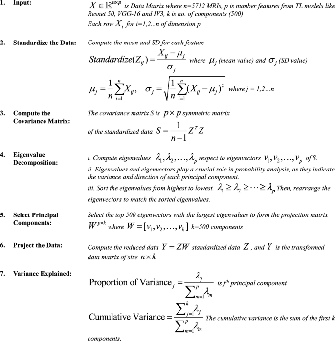
Eigenvectors and eigenvalues play a crucial role in probability analysis, as they indicate the variance and direction of each principal component. Cumulative variance analysis indicates that 500 components contribute significantly to the overall variance. Specifically, features from ResNet-50 account for 95.2% of the variance, while VGG-16 accounts for 94.8%, and Inception-V3 captures 95.0%. These findings are reasonable, considering the reduction of high-dimensional feature sets to 500 dimensions, as this process retains most of the information while minimizing noise.

The Table 4 details the learning rate schedule, batch size, and optimizer (Adam with β1 = 0.9 and β2 = 0.999), with an initial learning rate of 0.001 and a decay factor of 0.1 every 10 epochs.

MLP (100, 100) model

The Fig. 7 shows the MLP Model functionality. The MLP model has two hidden layers. It uses ReLU activations. This model is lightweight and powerful. It detects BTs. It uses softmax for classification. Forward propagation makes predictions by sending input through the MLP layers. Backward propagation updates the weights and biases based on the loss function’s gradient. An optimization algorithm, such as Adam is used to improve the weights.

The Multilayer Perceptron MLP (100, 100) Model is a powerful, lightweight model for detecting BTs, employing ReLU activations and softmax classification. It has an input layer with X and two hidden layers with 100 neurons and is trained using a categorical cross-entropy loss function.

1The MLP has an input layer. The input is a feature vector called X. This vector has n dimensions.

2 The MLP has two hidden layers. Each layer has 100 neurons. A formula defines the operation in each layer. This formula uses weights and biases to process inputs from the previous layer.

l denotes the layer index (1 or 2 for two hidden layers). \(W^{(l)} \in R^{m \times k}\) The weight matrix for layer l connects k neurons from the previous layer to m neurons in the current layer. H^(l−1) represents the output from the previous layer. For the first hidden layer, H⁽⁰⁾ equals X. The bias vector for layer l is denoted as b^(l). It belongs to the set of real numbers, R. The activation function is denoted by σ (it is the ReLU function).

The first hidden layer changes the input X. It creates a vector with 100 dimensions.

The second hidden layer changes H(1) into a new vector. This new vector has 100 dimensions.

3The Output Layer takes the results from the second hidden layer. It makes a single prediction. This prediction is for binary classification in tumour detection.

\(W^{(3)} \in {\mathbb{R}}^{2 \times 100} {\text{ and }}b^{(3)} \in {\mathbb{R}}^{2}\) It represents the weights of the output layer. b is a vector in R². It represents the biases of the output layer. The softmax function converts outputs into probabilities, determining the likelihood of each class, such as identifying tumours from those without them.

4The model is trained using a categorical cross-entropy loss function.

N represents the number of samples. ‘c’ indicates the number of classes. The true label is ( \(y_{i,c}\)). It is 1 if the sample belongs to class c and 0 otherwise. The predicted probability for class (c) is represented as \((\hat{y}_{i,c} )\).

Staking approach

A stacking ensemble learner combines predictions from multiple base models. It uses a meta-model to improve the final predictions. This method enhances generalization and accuracy. It is very effective for complex tasks, such as detecting BTs. Stacking has several advantages. It integrates the advantages of various base models. It helps improve overall performance. The meta-model can learn complex combinations of predictions. Stacking also reduces the risk of overfitting. A stacking ensemble has base models, also called Level-1 learners, which are represented by the ‘M’ f₁,f₂,f₃….f_M. Each base model (f_M) is trained separately. They use the training dataset. A meta-model is a type of model. It is called a Level-2 Learner. This model is trained using the predictions from base models. The logistic regression model in the stacking ensemble was improved through hyperparameter tuning. A grid search with tenfold cross-validation was used. The regularization parameter was set to C = 1.0. The solver chosen was ‘lbfgs’.

The training dataset is defined as eq. ()

X_i corresponds to the feature vector for the i^th instance. y_i is the true label for that instance. N indicates the total no. of instances. Stacking computational algorithm step by step as.

Step 1: The Base Model f_m is trained on the D dataset. \(\hat{y}_{i}^{(m)}\) is the prediction of the m^th base model for the ith instance.

Step 2: Meta-Features: The base models’ predictions are combined to create a new feature set called meta-features specific to each instance X_i. Z_i  ℝ^M represents the meta-feature vector for the i^th instance in ℝ.

Step 3: The Meta-Model g is trained on the meta-feature set {(Z_i,y_i)}, where i is the i^th instance and Z belongs to R is the meta-feature vector. The final prediction for the ith instance is represented

Step 4: The process for predicting a new instance X_new is as follows:

(i) The base models make predictions. They provide outputs based on their training.

A meta-feature vector is created as

(ii) The meta-model makes predictions. It determines as

Step 5: Optimization Objective: Base models minimize a loss function on the original dataset, ensuring accurate predictions and minimizing model impact on the original data, such as Mean Squared Error or Cross-Entropy.

Step 6: The meta-model reduces its loss function. It works on a set of meta-features. The function of loss is computed as the average of individual losses. Each loss compares the actual value to the predicted value from the model.

Performance parameters and confusion matrix

The confusion matrix (Fig. 8) evaluates BT classification performance by comparing predicted tumor types with actual tumour types across four classes: Pituitary Tumor (C1), No-Tumor (C2), Meningioma Tumor ((C4), and Glioma Tumor (C4). The dataset consists of diagonal entries representing correctly classified samples for each class and off-diagonal entries indicating misclassifications. Row totals represent the total number of predicted samples for each class, while column totals represent the actual number of samples for each class, regardless of their prediction. The overall total (T) is the sum of all samples in the dataset.

Accuracy refers to how closely an instrument’s measurements match a true value. It can be evaluated using small tasks and is calculated based on the proportion of correctly classified observations ³⁶.

Precision activity compares multiple measurements based on digital values, but accuracy must be considered in calculation, as illustrated in Eq. (2).

Recall is the ratio of correctly predicted positives based on all inspections in a class, as illustrated in Equation

The F1 score is calculated by combining the recall and precision scores, as illustrated in Equation