
Satellite payloads that include geostationary sensors, frequently detect long thin artificially created ship tracks in boundary layer clouds above large oceanic regions. These features are a result of the high concentrations of cloud condensation nuclei (CCN) that form from the nitrogen and sulfur oxides present in ship exhaust. In other words, the pollutants in ship exhaust can seed low-lying marine clouds by enhancing cloud droplet formation. However, because the clouds are water vapor limited, even in the marine boundary layer, cloud droplets, albeit more numerous, are typically smaller in clouds that have been influenced by ship effluents1. While suppression of droplet size may reduce the precipitation produced by marine clouds, the enhancement of droplet concentration from ship exhaust results in higher cloud albedo2,3. The microphysical process through which ship exhaust modulates cloud reflectivity is similar to a proposed climate adaptation strategy known as Marine Cloud Brightening (MCB)4, which is actively being studied as a potential solar climate intervention mechanism to slow down the impact of global warming, by reflecting more solar radiation back to space5,6,7,8,9. The study of ship tracks: satellite observable phenomena of natural MCB experiments, is thus critical in the development of MCB strategies.
The relatively bright tracks that may result from higher cloud albedos can persist for several hours after initial injection, before tracks fully disperse and become visibly indiscernible from other cloud features. However, it has been documented that a significant fraction of incoming solar energy reflected by tracks likely occurs over a longer lifetime (within 1-3 days after injection), with other studies indicating that clouds may take between a few hours to a few days to adjust and respond to aerosol injection5. In addition to determining the efficacy of MCB, the ability to quantify cloud responses to aerosol on varying timescales is crucial in furthering the scientific understanding of Aerosol-Cloud Interactions (ACI), poised as the largest source of uncertainty to global radiative forcing estimates10,11. Ship tracks, as natural experiments of aerosol injection, provide valuable insights into ACI by illustrating how aerosols influence cloud properties and behaviours12.
While expensive flight campaigns have historically enabled the bulk of high-resolution ACI measurement collection13,14, they are limited in data diversity; capturing spatio-temporal information from only small subsets of clouds that may cause difficulties in directly attributing aerosols to specific sources/times, and also presenting challenges for evaluating the spatio-temporal evolution of cloud parcels after injection. Thus, extracting similar measurements within satellite-measurable ship track regions could enhance the availability of data required for validation, though necessitate detailed and high-resolution representations of ship track regions which to the best of our knowledge, are not fully facilitated from current datasets.
The recent advent in field experiments of marine cloud aerosol injection15,16,17,18,19 to measure MCB efficacy, could directly benefit from quantitative comparison of realised cloud responses and brightening with those satellite-observed from ship tracks. Such comparisons, however, require a more complete understanding of track spreading. Ship track datasets which are currently available20,21,22 cannot be used to accurately measure track spreading, as they only provide partial information about coordinate label sets (i.e., a small set of spatial coordinates which tracks lie on). This is in contrast to the fully masked ship tracks presented in this paper, which provide gridded pixel locations covering all visible aspects of tracks.
While coordinate labels for tracks have shown promise in monitoring the density of ship tracks across the globe23,24, for more comprehensive analysis of the aerosol indirect effect and MCB efficacy, tracking the entire expanse of ship tracks is required25,26,27,28,29,30. For example, studies on how ship exhaust seeds existing clouds25, the formation and persistence of ship tracks in space and time31,32,33, when and where ship tracks are most apparent24, and their corresponding effects on cloud microphysics34, including insights into their overall climate forcing effects23, all necessitate the identification of fully masked ship tracks. Recent studies assessing the spreading behavior of tracks require complete track masks, especially of track edges, to compare changes in: strength, longevity, and spatial extent of cloud response and albedo, to those captured by new parameterizations of aerosol injection behavior33,35. In particular, ensuring the validity of such parameterizations against fully observed tracks would strengthen the ability to replicate cloud responses (and other aerosol indirect effects), thus having the potential to improve aerosol injection representation (that is currently poorly accounted for), in coupled climate models.
Despite requiring full tracks to measure track spreading rates via the calculation of changing plume widths (if visible) at different times after injection35, obtaining image masks of tracks is a challenging task. When visible, ship tracks appear distinct in certain satellite images (see Fig. 1), though they often resemble naturally forming cloud features with similar pixel intensities and textural attributes. As such, tracks cannot be separated from existing clouds through simple image manipulation or the determination of a pixel intensity threshold. Thus, although they can be distinct to human eyes, it is nontrivial to separate them from surrounding clouds. To this end, several semi-automated computational algorithms25,36,37 have been developed to extract pixels containing ship tracks from satellite imagery, using coordinate training data defining ship track locations (see e.g.34). Such algorithms in general utilise a thresholding approach to define regions of track vs no track, with thresholds and sizes of track regions chosen at fixed values, which may thus not necessarily cover all types of track lengths, features and trajectory shapes. Our proposed dataset aims to address this limitation by providing locations of tracks via pixel labels, allowing for more precise analysis and enhanced applicability. For instance, fully labelled ship tracks can be used directly as masks or rasters for other satellite data products beyond those which were used to create the labels, such as cloud liquid water path (LWP) as studied in37.

Examples of ship tracks as long thin streaks in clouds that become wider and more diffuse, around many other cloud features that are not always distinguishable as ship tracks. Raw images with projected (a) vs swath (b) taken by MODIS on July 15 2007 at 2:20 am in the North Pacific ocean, North East of Japan. Atmospheric Corrected Reflectance data plotted at the 2.1 μm band.
While there have been numerous studies of ship tracks utilising satellite imagery26,33, existing publicly available datasets of ship tracks only partially capture their intricate features, in comparison to the dataset we propose in this paper that fully captures tracks. As previously mentioned, for instance, the datasets of20,21 provide a list of latitude/longitude coordinates as track labels, as opposed to satellite image masks presented in this paper, which identify pixels representing ship tracks. Specifically, the 2019 ship track data of20 consists of a list of latitude/longitude coordinates corresponding to points that lie on the track’s centreline that runs adjacent to its (longer) side edges. Similarly, the 2022a dataset in21 labels each track over the years 2003-2020 by its date, time, mean latitude, and mean longitude; computed over all the pixels that are machine-learned as representing ship tracks. The dataset does not contain the image masks corresponding to the machine-labelled pixels representing ship tracks, nor the hand-labelled training dataset used to train the machine learning algorithm described in23. On the other hand, the 2022b ship track dataset provided and utilised in24 provides both hand-labelled training38 and derived machine learned data22, in the form of centreline polygon masks representing latitude/longitude coordinates of a polygon encapsulating the central region of each ship track. From the references therein, the utilised training data leverages an unpublished ship track dataset, first mentioned in34, that highlights hand logged labels consisting of a latitude/longitude coordinate corresponding to the head, or most recently formed part of the track, and each coordinate representing a track’s turning point wherein it abruptly changes direction to form its quasi-linear structure. The centreline polygon masks are then obtained by connecting each of these hand-labelled coordinates by straight lines separated by a static width of 10 pixels (approximating the average ship track width of 9 km), in which the centreline corresponds to the line separating the polygon in half. Figure 2 visualises the differences in track labelling amongst the datasets that currently exist, and the dataset we present that aims to mask the entirety of track features.

Example of current databases’ masking techniques against the masking technique used in our proposed dataset. Track observed on June 15 2006 at 6:45 pm.
The unpublished hand-labelled dataset of34, highlighting track head and turning point coordinates, has since been either directly utilised or added to in many subsequent ship track studies36,37,39. In particular, the dataset utilised in36 is the 2019 dataset20 that we study in this paper. To visualise these differences in a full satellite image, Fig. 3 shows the same image as Fig. 1 with now labelled tracks in the form of: centreline coordinates (as shown by the 2019 dataset of20), a mean coordinate (as given in the 2022a dataset of21), centreline polygon marks (as given in the 2022b dataset of38), and satellite masks consisting of all pixels that contain a track (our contribution).

Swath MODIS image containing ship track labels from Watson-Parris et al. (shown in green)38, Song et al. (shown in red)21 and Toll et al. (shown in black)20 shown against our proposed data masks (shown in orange). Image taken July 15 2007 at 2:20 am in the North Pacific ocean, North East of Japan.
Curating a new dataset of ship track image masks during this specific time period is important for multiple reasons. First, both optimising the efficacy of MCB for maximum solar reflectivity and benchmarking varied observations of ACI, requires understanding of the atmospheric conditions leading to ship track formation and maximal persistence. However, formation of ship tracks itself is heavily dependent on the amount of sulphur contained in their corresponding emissions that can viably produce small enough droplet sizes when seeded, to be discernible from the surrounding clouds by satellite23. Notably, sulphur oxides have seen more stringent regulations over the past decade, particularly in specified emission control areas (ECAs), to minimise the negative impacts of airborne ship emissions. These regulations have led to a significant decline in observable ship tracks since 201023,24. As a result, there is strong evidence to suggest that studying ship tracks before the first restrictive policy in 2010 provides a more robust understanding of track formation, persistence and spreading, given their higher probability of formation, detection and discernibility.
Before 201023, show that the year 2006 provides the highest ship track density in the North Pacific and South East Atlantic regions, containing the majority of globally observed ship tracks, both inside and outside of ECAs. Further, tracks detected in the Northeast Pacific prior to 2009 produce the largest difference in cloud droplet number concentration between track and background since 200323, optimising their satellite discernibility and utility for studying MCB efficacy. For these reasons, we choose to look at tracks around the 2006 period to create a dense dataset of tracks in varied regions globally.
The MODIS observations were selected from NASA’s Earth Data repository1. The collection was influenced by those compiled in20, with the days selected intended to contain images where ship tracks were numerous and highly visible. The 2019 dataset of20 provides the dates and times of ship track instances, and a list of longitude and latitude coordinates along the centreline of each ship track.
The dataset provided in this paper can be used to build predictive models for automating the masking of unlabelled ship tracks from other images. Without an intermediate model to convert provided labels to image masks, building such predictive models is not straightforward using labels which consist of lists of latitude/longitude coordinates, centrelines, centreline polygon regions or mean coordinates, as provided in the publicly available datasets20,21,38. Training automated predictive models which label pixels in images as ship tracks typically requires training data which corresponds to the desired output format, namely, image masks which identify exactly which pixels in an image represent ship tracks. The dataset provided here contains such image masks, and can be used directly for training Machine Learning models which automatically generate new image masks for unlabelled images. With these masks, we additionally provide key track metadata including coordinates of their emission points, angles and centrelines, intended to provide further quantitative descriptors of each track for such downstream analyses.
Summary
We develop a hand-labelled dataset conveying full ship track trajectories in the form of image masks, using data from the MODIS (Moderate Resolution Imaging Spectroradiometer) instrument. To the best of our knowledge, our dataset40 providing full image masks representing ship tracks on images from MODIS is first-of-its-kind. The dataset is comprised of 300 separate MODIS observations over a span of time between June 15, 2006 and August 20, 2007: a period stretching more than a year with a total of 2,543 ship tracks present in the data.
The images were selected to cover a range of geographical locations, primarily over the North Pacific and South Atlantic oceans, where ship tracks are frequently observed. Further, the images are not evenly distributed in time and location but are concentrated in regions and seasonal periods where ship tracks are most likely to form. Specifically, the majority of images cover areas along known shipping lanes with high traffic, such as the North Pacific, the South Atlantic, the west coast of southern Africa, and the west coast of South America, under suitable atmospheric conditions for ship track formation. Studies have shown these conditions are primarily due to seasonal changes in the abundance of very low clouds, prevalent during warmer months (e.g., May-July in the Northern Hemisphere)41.
To summarise the data generation and validation process: we started by compiling the MODIS observations tagged in the 2019 dataset of20, as those containing ship tracks. Each of these observations were then validated by eye from a human labeller, and those with no obvious ship tracks discarded. Next, the observations were visualised in their raw form, i.e. without any projections, and pixels containing ship tracks masked in full, via their distinct features. This masking was done using the data’s non-projected form, to ensure that the masks would be able to be projected into every other format necessary. Since each projection may differ slightly, the most universal format was used for the foundational masking. Once the masks were conceived, they were validated by two other labellers, with ship track pixels not determined by the other two labellers discarded. Subsequently, we post-processed the hand-labelled masks to extract additional track statistics: including automatically computed track centrelines, track heads, and corresponding orientation angles. Finally, the dataset was complied, consisting of:
-
Raw (unprojected) directory: Containing unprojected raw image data and the corresponding masks/rasters.
-
Padded directory: Containing raw padded data and padded masks/rasters.
-
Projected directory: Containing projected image data onto a flat latitude/longitude grid using the plate Carrée projection with interpolated values being either the minimum (min) or interpolated (interp), and the corresponding projected masks/rasters.
-
Swath directory: Containing image data visualised as a MODIS swath and the corresponding swath-visualised masks/rasters.
-
Metadata: A JSON file providing additional track statistics, including the computed centrelines, track head coordinates, and orientation angles.
Footnote 1
The process of the dataset creation and validation is outlined in Fig. 4, where the masking described can be situated within the larger context of the outputted image data products, provided in the finalised dataset.
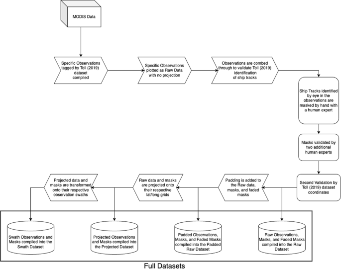
The full process of our proposed dataset creation from initial masking to the compilation of the various datasets we provide.
We use the datasets of20,21,38 to validate our ship track masks and labelling methodology. More details about the validation process are provided in the Technical Validation section.


