A Fig. 1 provides an overview of the proposed system for MSD. It integrated three modules involving Detection algorithm, mature strawberry detection and a deployment. This integrated strategy addresses the challenges of accurate and real-time crop monitoring. The deployment was carried out in both simulation and real-time modes to validate the proposed algorithm.

The Strawberry detection architecture is deployed on a quadrotor system for practical, real-world applications. The quadrotor system includes a camera to facilitating automated crop monitoring of strawberry plants
Detection model
Effective crop monitoring is essential prior to harvesting ripe strawberries. To accurately detect ripe strawberries, it is crucial to first study the fruit’s classes (unripe and ripe) to collect corresponding data. This dataset serves as the foundation for training an accurate detection model. In Fig. 2 represents a strawberry classes (a) an unripe fruit, and (b) a fully ripe fruit.
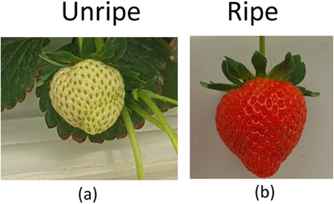
Strawberry fruit. a an unripe fruit, and b a fully ripe fruit
Strawberries, cherished for their vibrant color, sweet flavor, and rich aroma, are not only a popular fruit worldwide but also a powerhouse of nutrients. Given their delicate structure, perishable nature, and visual cues associated with ripeness, strawberries are an ideal candidate for precision agriculture applications. Computer vision technologies can significantly aid in monitoring plant health, assessing fruit maturity, and automating harvest timing. By integrating AI-powered systems into strawberry farming, growers can optimize yield, reduce labor costs, and ensure consistent fruit quality, ultimately promoting sustainable and efficient agricultural practices.
Dataset
A quadrotor was utilized to capture crop data in video format during flying over the crop, and the detection model was later applied in offline mode to analyze the number of ripe strawberries. In this study, we utilized a dataset comprising 250 images from a CAD-based synthetic dataset and 800 images for real strawberries in greenhouse. The variation in the dataset enhance the model performance validity. So, total 1050 images were used in dataset. The dataset consisted of one class: ripe strawberries (0). The domain randomization technique is applied on the images by variations in brightness, different backgrounds, and shaded areas. Table 1 provides comprehensive details about the images contained within the dataset. To enhance training data diversity, various augmentation methods were implemented, including rotation, flipping, and blurring transformations. These techniques contribute to strengthening the model’s generalization capabilities across diverse operational conditions. The dataset was divided using a standard 70:20:10 split ratio, allocating 735 images for training, 210 images for validation, and 105 images for testing. This distribution ensures sufficient training data while maintaining adequate validation and test sets for reliable performance evaluation.
Figure 3 presents a comparative view of both the actual strawberry farm image dataset environment and the synthetic Gazebo environment generated through CAD methodology using Blender software. Within this dataset, mature strawberries exhibit distinctive features including a rich red coloration, smooth texture, and substantial, well-developed fruit size. These defining characteristics serve as essential indicators for determining strawberry maturity and provide valuable resources for researchers and developers working on automated strawberry ripeness detection systems, ultimately contributing to improved operational efficiency and product quality in the strawberry cultivation industry.
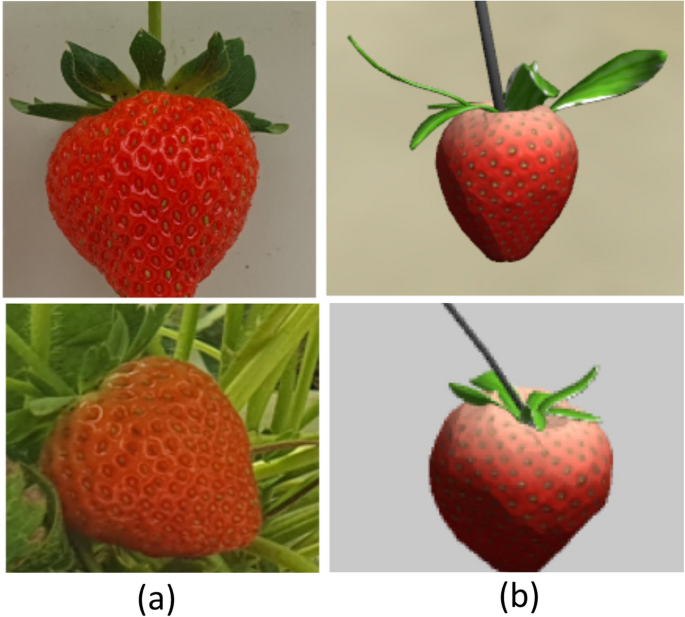
Image dataset collection environments (a) Real ripe strawberries dataset, and (b) CAD synthetic ripe strawberries dataset created using Blender software
The Computer Vision Annotation Toolbox (CVAT) was used for markup. It allows you to make annotations in various formats. Figure 4 shows an example of data markup in CVAT [36].
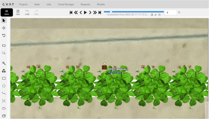
Image dataset collection environments (a) Real ripe strawberries dataset, and (b) CAD synthetic ripe strawberries dataset created using Blender software
Detection model architecture
Conventional image analysis techniques rely on scanning datasets through numerous sliding windows to extract pertinent features, followed by classifier implementation for object identification. To enhance the effectiveness of this methodology, researchers developed a CCL-SVM framework [71] utilizing Support Vector Machine algorithms specifically designed for identifying diseases in tomato foliage, particularly under complex and demanding environmental conditions. A fruit detection and quality assessment system based on YOLOv5 was introduced by Goyal (2022) [23], operating through a two-phase process. The primary detection stage attained a mean Average Precision of 92.80% for identifying fruits. During the quality analysis phase, the model recorded mAP scores of 99.60% and 93.10% for apples and bananas respectively. This method proved highly effective in automated fruit sorting applications, consistently producing accurate classification results. An innovative strawberry ripeness assessment technique was presented by Yang (2023) [70], which merged YOLOv8 with the LW-Swin Transformer for improved detection capabilities. The team modified the feature fusion network by integrating a residual structure containing learnable parameters and scaled normalization elements into the standard Swin Transformer design. Validation results confirmed that their proposed LS-YOLOv8s model substantially exceeded competing methods, demonstrating mAP@0.5 improvements of 1.6% over YOLOv5s, 33.5% over CenterNet, and 3.4% over SSD during experimental evaluation.
In our research we are using YOLOv9 base model instead of the more recent YOLOv10, v11, or v12 due to following reasons:
-
YOLOv9 introduces a strong balance between accuracy, inference speed, and model size, making it suitable for real-time embedded or edge deployments. While YOLOv10–v12 may have improved accuracy, they often come with increased computational complexity or larger model sizes that are not ideal for all environments (e.g., low-power robots, drones, IoT devices) [66]
-
In our tasks such as (e.g., greenhouse strawberry detection using both synthetic CAD and real images), YOLOv9 handles domain shifts effectively due to its strong generalization in mixed-data scenarios.
The research proposes a new architectural concept known as Generalized ELAN (GELAN), representing an advanced iteration of the original ELAN framework [25]. By integrating CSPNet and ELAN concepts, GELAN enables strategic gradient pathway management. The architecture’s development focuses on achieving minimal computational overhead, accelerated inference performance, and enhanced accuracy levels. The overall architecture of GELAN is depicted in Fig. 5. To assess GELAN’s effectiveness, we performed experiments using a mixed dataset containing both synthetic CAD-generated images and real strawberry photographs. These experiments took place in a controlled gazebo greenhouse setting. The experimental findings demonstrated that our proposed YOLOv9 model outperformed all other compared models across every evaluation metric tested.
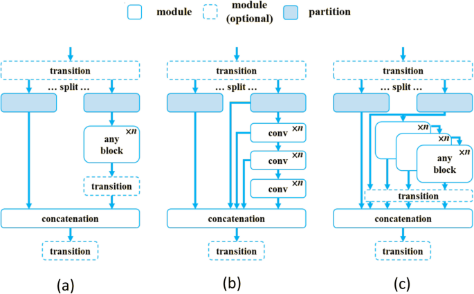
The architecture of GELAN: a CSPNet, b ELAN, and c GELAN [66]
In this study, we trained and validated a detection model using an enhanced YOLOv9 architecture integrated with the GLEAN framework for strawberry crop monitoring applications. As shown in Fig. 6, the YOLOv9-GELAN architecture is structured into three primary components: the backbone, neck, and head. The model accepts input images of size 640 \(\times\) 640 \(\times\) 3, representing RGB color channels. Initially, two convolutional blocks with a kernel size of 3 and a stride of 2 are applied to reduce the spatial resolution. The number of channels in these convolution blocks varies based on the configuration of the YOLOv9 architecture.
The output from the initial convolution layers is passed to the RepNCSPELAN block, which defines the number of replications and bottleneck blocks used. Additionally, an ADown block is employed for downsampling, further reducing the feature map resolution. At the end of the backbone, the RepNCSPELAN block connects to the SPPELAN (Spatial Pyramid Pulling Efficient Layer Aggregation Networks) block. In the neck section, the SPPELAN output is upsampled to align with the feature map resolution of the RepNCSPELAN block using an Upsample block. A Concat block then merges the features from both the Upsample and RepNCSPELAN blocks by summing the channel values while preserving spatial dimensions. This alignment ensures that the feature resolutions from both the backbone and neck components are consistent. Subsequently, the feature map is forwarded to the head of the architecture, which consists of three detect blocks.
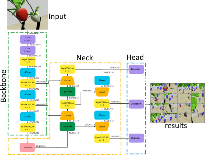
YOLOv9-GELAN architecture for strawberry detection, featuring a backbone network (green) for feature extraction through RepNCSPELAN blocks, a neck network (yellow) with Feature Pyramid Network for multi-scale feature fusion, and detection heads (blue) that output precise bounding boxes for ripe strawberry detection
Each block is designed to handle objects of different sizes: small, medium, and large. These blocks operate on feature maps with a resolution of 20 \(\times\) 20 \(\times\) 512. The training is done for 300 epochs with batch size 16 and image size 640.
Training process
The network training for this research was conducted using a hardware setup that included an Intel(R) Core(TM) i9-14900KF processor operating at 3.20 GHz, 128 GB of system memory, a 2 TB hard disk drive, and an NVIDIA GeForce RTX 3090 graphics processing unit. Ubuntu served as the operating system platform, with PyTorch functioning as the deep learning framework. The software environment comprised Python version 3.9.18, torch-2.1.2+cu118, and OpenCV 3.4.5. Training was performed on YOLOv9-GELAN, YOLOv9, and YOLOv8 models using input images scaled to 640 x 640 pixels. The training configuration employed a starting learning rate of 0.001, momentum parameter of 0.90, weight decay coefficient of 0.0005, and a batch size of 16 samples. All models underwent training for 300 epochs, with multiple iterations through the complete dataset to achieve optimal model performance.
The trained model was evaluated on validation dataset using various evaluation metrics to assess their performance. These metrics included precision (P), recall (R), F1 score, average precision (AP), and mean average precision (mAP). The Mean Average Precision (mAP) statistic is often used to evaluate object-detecting algorithms. This measure is computed by comparing predicted bounding boxes to their corresponding ground truth bounding boxes. The Intersection Over Union (IoU) is an important component of this comparison since it evaluates the overlap between the anticipated bounding box and the ground truth.
$$\begin{aligned} IoU=\frac{\text {area of overlap}}{\text {area of union}} \end{aligned}$$
(1)
Precision is the proportion of true positives out of all the positive predictions made by a model. It measures how accurate the model’s positive predictions are.
$$\begin{aligned} Precision = \frac{\text {True Positives}}{\text {True Positives} + \text {False Positives}} \end{aligned}$$
(2)
Recall is the proportion of true positive samples that the model correctly identified as positive out of all the true positive samples. In other words, recall measures how well the model is able to find or detect the positive samples. A higher recall value indicates the model is able to correctly identify a larger proportion of the actual positive cases.
$$\begin{aligned} Recall=\frac{\text {True Positives}}{\text {True Positives} + \text {False Negatives}} \end{aligned}$$
(3)
The F1 score combines these two factors into a single value that indicates how well the model can accurately predict outcomes. An improved ability to balance accurately detecting instances that are positive with reducing false positives is shown by a higher F1 score for the model. To summaries, the F1 score evaluates a classification model’s overall efficacy by considering its precision (accuracy in producing positive predictions) and recall (ability to identify positive occurrences). It is a useful metric for evaluating how well a model can anticipate outcomes.
$$\begin{aligned} F1_{score}= 2 \times \frac{Recall \times Precision}{Recall + Precision} \end{aligned}$$
(4)
Figure 7 illustrated the confusion matrix for proposed strawberry detection model YOLOv9-GLEAN and other baseline models YOLOv8 and YOLOv9, comparing their performance in classifying ripe strawberries versus background elements. Each matrix displays the relationship between true labels (horizontal axis) and predicted labels (vertical axis) for binary classification tasks. Figure 7a shows the YOLOv8 model’s performance with 735 total predictions. The model correctly identified 711 ripe strawberries (true positives) and misclassified 22 ripe strawberries as background (false negatives). Additionally, 3 background elements were incorrectly classified as ripe strawberries (false positives). This demonstrates high sensitivity for ripe strawberry detection with minimal false positive errors. Figure 7b presents YOLOv9 performance with 735 total predictions. The model achieved 719 correct ripe strawberry classifications (true positives) with only 15 false negatives, representing better recall compared to model Fig. 7a. The false positive rate remained extremely low with only 1 background misclassifications, indicating enhanced precision. Whereas, Fig. 7c exhibits the best overall performance (proposed YOLOv9-GLEAN) with 735 predictions. This model correctly classified 724 ripe strawberries (highest true positive rate) while reducing false negatives to just 10 cases. The false positive rate remained minimal with only 1 background misclassifications, demonstrating optimal balance between precision and recall.
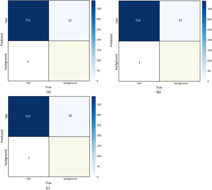
Confusion matrix a YOLOv8, b YOLOv9, and c YOLOv9-GLEAN
The training progress analysis reveals exceptional performance of the YOLOv9-GLEAN based strawberry detection model across 200 epochs of training. Figure 8 illustrated the training process performance parameters. The localization accuracy improved significantly, with the training box loss decreasing from an initial value of 2.6 to a final converged value of 1.0, while the validation box loss demonstrated similar improvement from 6.0 to approximately 1.0, indicating robust generalization capabilities. Classification performance showed remarkable convergence, with training classification loss rapidly declining from 28 to near-zero within the first 50 epochs, and validation classification loss exhibiting even more dramatic improvement from 140 to essentially zero. The Distribution Focal Loss (DFL) metrics further confirmed model reliability, with training DFL loss reducing from 2.2 to 1.7 and validation DFL loss decreasing from 7.0 to 1.8, demonstrating improved confidence calibration throughout the training process.
The performance metrics underscore the model’s exceptional detection capabilities, with precision rapidly ascending from 0.2 to nearly 1.0 within the initial 25 epochs and maintaining this high level throughout training. Recall performance followed a similar trajectory, achieving near-perfect scores of 1.0 early in training and sustaining this performance consistently. The mean Average Precision at IoU threshold 0.5 (mAP50) reached outstanding values of approximately 1.0, while the more stringent mAP50-95 metric, which evaluates performance across multiple IoU thresholds from 0.5 to 0.95, achieved impressive scores of 0.95. These metrics demonstrate that the model achieved rapid initial learning within the first 25-50 epochs, followed by stable convergence without signs of overfitting, making it highly suitable for real-world automated strawberry detection and monitoring applications in agricultural settings.
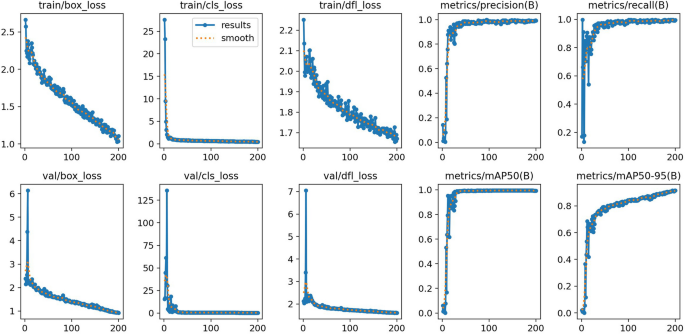
Training process performance parameters
Figure 9 illustrated the performance evaluation of the trained model. As depicted in Fig. 9 the model demonstrates exceptional performance in detecting ripe strawberries in video frames captured by quadrotor, achieving near-perfect precision and recall. In Fig. 9a F1-confidence curve indicates that the best balance between precision and recall occurs at an F1-score of 0.99 at a confidence threshold of 0.471.
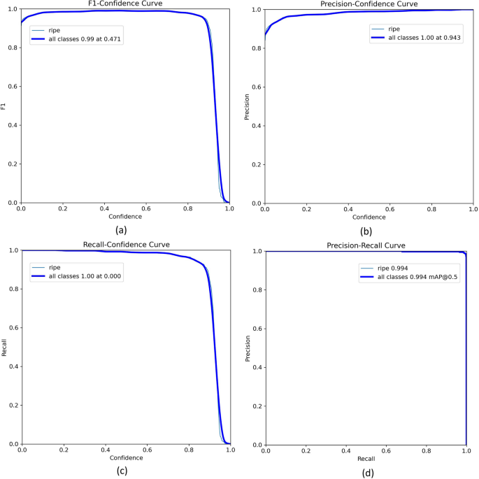
Performance evaluation curves for YOLOv9-GELAN strawberry detection: a F1-confidence achieving 0.99 at threshold 0.471, b precision-confidence reaching 1.00 at 0.943, c recall-confidence maintaining 1.00 until 0.8 threshold, and d precision-recall curve with exceptional mAP@0.5 of 0.994, demonstrating superior detection performance
The precision-confidence curve reveals that the model achieves a precision of 1.00 at a confidence threshold of 0.943 as per Fig. 9b, suggesting that when the confidence threshold is high, the model makes highly precise predictions with minimal false positives. In Fig. 9c the recall-confidence curve shows that the model attains 1.00 recall at a confidence threshold of 0.000, meaning it detects all ripe strawberries at low thresholds but may also include false positives. The precision-recall curve (Fig. 9d) further confirms the model’s robustness, achieving a mean average precision (mAP@0.5) of 0.994, highlighting its high effectiveness in crop monitoring applications.
YOLOv9 extends the capabilities of YOLOv8 through the integration of advanced architectural components, including CSPNet (Cross-Stage Partial Networks) and ELAN (Efficient Layer Aggregation Networks). These components enhance the network’s capacity to achieve an optimal balance between computational efficiency and detection accuracy across multiple object scales. CSPNet facilitates improved gradient propagation during the backpropagation process, resulting in more efficient learning while maintaining performance integrity. Meanwhile, ELAN enhances feature aggregation across different network layers, thereby strengthening overall feature extraction capabilities from input imagery. The key innovation in YOLOv9-GELAN lies in the incorporation of GELAN, which empowers the model to produce high-resolution image features that significantly enhance detection precision. This advancement proves particularly valuable for strawberry detection applications, where subtle visual characteristics such as color variations, surface texture, and fruit dimensions are critical for accurate ripeness classification. This capability is essential for strawberry detection in complex scenarios, including cluttered environments or reduced-quality images commonly encountered in greenhouse settings.
The precise details of the metrics and their respective scores can be found in Table 2. These results suggest that the YOLOv9-GELAN model is more effective and robust in accurately detect tiny objects.
According to the findings in Table 2, the YOLOv9-GELAN model demonstrated superior performance compared to the other available models. YOLOv9-GLEAN achieves a precision of 0.991 and recall of 0.990, outperforming previous and latest versions and also have more FPS (offline processing speed). The ability to better differentiate strawberries from the background is enhanced by GLEAN’s super-resolution capability, reducing false positives and negatives.
Quadrotor modeling
Although this study primarily focused on developing the MSD (Mature Strawberry Detection) algorithm for robust detection of ripe strawberries, our main research objective is to integrate this algorithm into a quadrotor platform to be used for greenhouse crop monitoring. Two main components of this robotic system include a system modeling, and hybrid trajectory tracking controller.
System modeling
Defining the coordinate frames is the first step in modeling quadrotor dynamics. Figure 10 shows the frames define in the quadrotor modeling. The quadrotor will operates in two frames (i) inertial frame \((\textrm{x}_{i},\textrm{y}_{i},\textrm{z}_{i})\) and body frame \((\textrm{x}_{b},\textrm{y}_{b},\textrm{z}_{b})\). The inertial frame is defined relative to the ground, with the positive z-axis oriented upward. In contrast, the body frame is defined with respect to the quadrotor’s center of gravity, and its axes are fixed to the body of the quadrotor. The governing equation is derived by using projection matrices to transform quantities between the two frames [27]. Coordinate frame transformations are used to convert quantities between two reference frames. The quaternion method is employed to perform these transformations efficiently and accurately [34]. The coordinate transformation between two distinct reference frames is calculated using quaternion rotation as [22].
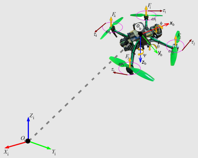
Quadrotor diagram and its reference frames
$$\begin{aligned} A = q \otimes A^{‘} \otimes q^{-1} \end{aligned}$$
(5)
Here, \(\textrm{A}\) represents the rotated vector, and \(\textrm{A}^{‘}\) is the vector to be rotated. Equation 1 indicates that multiplying two or more rotation quaternions yields another quaternion. In pure quaternions, vectors can be transformed between frames by first converting them into quaternions with a zero scalar component. Thus, the quaternion-based rotation matrix that maps the inertial frame to the body frame can be derived by reformulating Eq. (5) as follows:
$$\begin{aligned} \left[ \begin{array}{c} 0\\ r_{b} \end{array} \right] = q \otimes \left[ \begin{array}{c} 0\\ r_{i} \end{array} \right] \otimes q^{*} \end{aligned}$$
(6)
whereas \(\textrm{r}_{b}\) = \([\textrm{x}_{b},\textrm{y}_{b},\textrm{z}_{b}]^{‘}\) and \(\textrm{r}_{i}\) = \([\textrm{x}_{i},\textrm{y}_{i},\textrm{z}_{i}]^{‘}\) are position quantities with respect to body frame and inertial frame respectively. The 3D rotation matrix \(\textrm{R}_{B}^{I}\left( q \right)\) for position projection from body frame to inertial frame is obtained using Eq. (6) as follows [54]:
$$\begin{aligned} \left[ \begin{array}{c} x_{i}\\ y_{i}\\ z_{i}\end{array} \right] = \left[ \begin{array}{lll} 2\left( q_{o}^{2} +q_{1}^{2}\right) -1 & 2\left( q_{1}q_{2} + q_{0}q_{3}\right) & 2\left( q_{1}q_{3}-q_{0}q_{2} \right) \\ 2\left( q_{1}q_{2} – q_{0}q_{3}\right) & 2\left( q_{o}^{2} +q_{2}^{2}\right) -1 & 2\left( q_{2}q_{3}+q_{0}q_{1} \right) \\ 2\left( q_{0}q_{2}+q_{1}q_{3} \right) & 2\left( q_{2}q_{3}-q_{0}q_{1} \right) & 2\left( q_{o}^{2} +q_{3}^{2}\right) -1 \end{array}\right] \left[ \begin{array}{c} x_{b}\\ y_{b}\\ z_{b}\end{array} \right] \end{aligned}$$
(7)
The transformation matrix that projects the body frame rates \(\omega =\left[ \begin{array}{ccc}p&q&r \end{array}\right] ^{‘}\) into the inertial frame rates \(\mathrm q\dot{}\) can be derived as follows [9]:
$$\begin{aligned} \left[ \begin{array}{c} q\dot{}_{0} \\ q\dot{}_{1} \\ q\dot{}_{2} \\ q\dot{}_{3} \end{array}\right] = \frac{1}{2}q\otimes \omega = \frac{1}{2}\left[ \begin{array}{cccc} q_{0} & -q_{1} & -q_{2} & -q_{3} \\ q_{1} & q_{0} & -q_{3} & q_{2} \\ q_{2} & q_{3} & q_{0} & -q_{1} \\ q_{3} & -q_{2} & q_{1} & q_{0} \end{array}\right] \left[ \begin{array}{c} 0 \\ p \\ q \\ r \end{array}\right] \end{aligned}$$
(8)
The following assumptions were made to model the quadrotor flight dynamics within the greenhouse environment.
-
Quadrotor is rigid body with fixed mass and uniform symmetry.
-
No external disturbance (wind) in the controlled greenhouse environment.
-
Constant gravitational force.
-
Motor resistance \(\textrm{m}_{r}\) is negligible.
-
Pre-defined way points for quadrotor trajectory.
By defining the angular velocities for the four rotors of quadrotor as \(\omega _{1},\omega _{2},\omega _{3},\omega _{4}\), the total lift in the Z direction of body frame as \(\textrm{T}_{L}\), and the torques around body frame axis as \(\tau _{x},\tau _{y},\tau _{z}\), and then it can be obtained as:
$$\begin{aligned} T_{L}=L_{c}\left( \omega ^{2}_{1}+ \omega ^{2}_{2}+\omega ^{2}_{3}+\omega ^{2}_{4}\right) \end{aligned}$$
(9)
$$\begin{aligned} \tau _{x}=lL_{c}( \omega ^{2}_{2}-\omega ^{2}_{4} ) \end{aligned}$$
(10)
$$\begin{aligned} \tau _{y}=lL_{c}( -\omega ^{2}_{1}+\omega ^{2}_{3}) \end{aligned}$$
(11)
$$\begin{aligned} \tau _{z}=b( -\omega ^{2}_{1}+\omega ^{2}_{2}-\omega ^{2}_{3}+\omega ^{2}_{4}) \end{aligned}$$
(12)
Here, \(\mathrm {\textit{L}_{c}}\) represents the lift coefficient, \(\mathrm {\textit{b}}\) denotes the anti-torque coefficient, and \(\mathrm {\textit{l}}\) corresponds to the length of the quadrotor arm. The model of the quadrotor is calculated as:
$$\begin{aligned} \ddot{x}=\frac{1}{m}\left[ T_{L}\left( cos\phi sin\theta cos\psi + sin\phi sin\psi \right) -d_{c}\dot{x}+F_{dx} \right] \end{aligned}$$
(13)
$$\begin{aligned} \ddot{y}=\frac{1}{m}\left[ T_{L}\left( cos\phi sin\theta sin\psi – sin\phi cos\psi \right) -d_{c}\dot{y}+F_{dy} \right] \end{aligned}$$
(14)
$$\begin{aligned} \ddot{z}=\frac{1}{m}\left[ T_{L} cos\phi cos\theta -d_{c}\dot{z}-mg+F_{dz} \right] \end{aligned}$$
(15)
$$\begin{aligned} \dot{\phi }=p+q sin\phi tan\theta +r cos\phi tan\theta \end{aligned}$$
(16)
$$\begin{aligned} \dot{\theta }=q cos\phi -rsin\phi \end{aligned}$$
(17)
$$\begin{aligned} \dot{\psi }=\frac{1}{cos\theta }(q sin\phi +rcos\phi ) \end{aligned}$$
(18)
$$\begin{aligned} \dot{p}=\frac{1}{I_{xx}}\left[ \left( I_{zz}-I_{yy} \right) qr+\tau _{x}+\tau _{dx} \right] \end{aligned}$$
(19)
$$\begin{aligned} \dot{q}=\frac{1}{I_{yy}}\left[ \left( I_{xx}-I_{zz} \right) pr+\tau _{y}+\tau _{dy} \right] \end{aligned}$$
(20)
$$\begin{aligned} \dot{r}=\frac{1}{I_{zz}}\left[ \left( I_{yy}-I_{xx} \right) qp+\tau _{z}+\tau _{dz} \right] \end{aligned}$$
(21)
where x,y,z denotes the position in inertial frame, m mass of quadrotor, g is the gravity, \(d_{c}\) is drag coefficient; \(\phi\),\(\theta\),\(\psi\) represent the roll, pitch and yaw angle, p,q,r denotes the angular rates around body frame, \(I_{xx}\), \(I_{yy}\), and \(I_{zz}\) are moments of inertia; \({F_{dx}}\), \(F_{dy}\), \(F_{dz}\) are external disturbance forces, and \(\tau _{dx}\), \(\tau _{dy}\), \(\tau _{dz}\) denotes the external disturbance torques. In our case external disturbance forces and torques are negligible due to control environment of the greenhouse. Using Eqs. (13) to (21), a MATLAB-Simulink model was developed, as shown in Fig. 11.

Simulink model of 6 dof quadrotor for predefine way-points
Table 3 mentioned the hardware specifications of the quadrotor deployed for mature strawberry detection application.
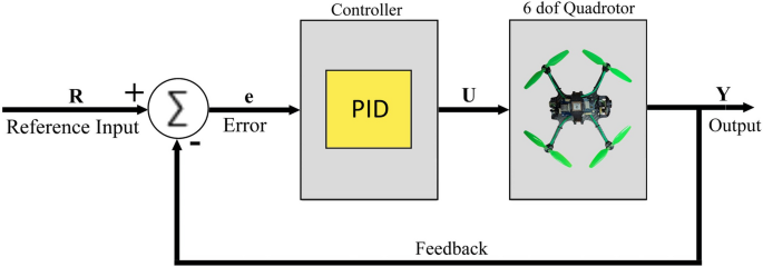
Closed loop PID controller for Quadrotor system
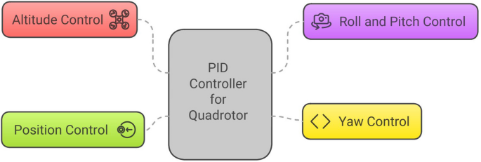
Overall PID controller for quadrotor comprises of sub-control modules i.e. altitude control, roll and pitch control, position control, and yaw control
Trajectory tracking controller design
Research in quadrotor controller design is a rapidly growing field driven by the rising demand for autonomous drones in areas such as delivery, surveillance, agriculture, and disaster response. Developing robust and efficient controllers for quadrotors presents significant challenges, including managing nonlinear dynamics, under-actuation, axis coupling, and external disturbances like wind. Controllers like PID [37, 53], Adaptive PID [39], LQR [17, 40], and MPC [18, 29] are extensively utilized for controlling linear and nonlinear quadrotor systems. In our work, no external disturbances, such as wind, are present since the greenhouse provides a controlled environment. Therefore, we proposed robust controller using classical PID and optimal LQR for the quadrotor, as they are simple and easy to implement on the system. Combining PID and LQR controllers for quadrotor control offers both robustness and optimal performance. The proposed controller is designed to first achieve the target position in the Z direction (maintaining a constant height) and then follow the predefined way-points for scanning strawberry plants within the greenhouse.
-
PID controller Designing a PID controller for a quadrotor requires managing its motion across multiple axes, including roll, pitch, yaw, and altitude. A quadrotor has six degrees of freedom (DOF): three translational (x, y, z) and three rotational (roll, pitch, yaw). The PID controller plays a crucial role in stabilizing and regulating these movements. The PID controller is a classic model in control theory, designed to minimize errors by adjusting the proportional, integral, and derivative coefficients in the quadrotor control equation. Figure 12 depicts the closed loop PID controller for quadrotor system. The proportional term adjusts the error by multiplying it with a proportionality constant, either increasing or decreasing the response. The derivative term predicts the controller’s future behavior by analyzing the rate of change of error over time. The integral term accumulates all past error values, with the integral coefficient determining its influence to achieve the desired output in the shortest time. Therefore, tuning coefficients proportional, integral, and derivative is essential to reach the control system’s set-point effectively. Error (e) is defined as the difference between the reference input (R) value and the output of the system (Y) at any given moment. The output of the controller (U) is fed to the quadrotor system as input. The overall PID controller for the quadrotor comprises sub-control modules, including altitude control, roll and pitch control, position control, and yaw control, as illustrated in the Fig. 13. The general PID control equation is given below: whereas \(\mathrm {\textit{U}{
(22)
The force in the upward Z-axis is given by:
$$\begin{aligned} F_{z}=m\ddot{z}+mg \end{aligned}$$
(23)
where: \(\mathrm {\textit{F}_{z}}\) is the total thrust force along Z-axis, \(\mathrm {\textit{m}}\) is the mass of the quadrotor, \(\mathrm {\ddot{\textit{z}}}\) is the upward acceleration, and \(\mathrm {\textit{g}}\) is the gravitational acceleration. The control objective is to regulate the altitude (z) to track a desired altitude value (\(\mathrm {\textit{z}_{desired}}\)). The altitude error is defined as:
$$\begin{aligned} e_{z}=z_{desired}-z_{actual} \end{aligned}$$
(24)
The control force (\(\mathrm {\textit{F}_z}\)) must be designed to ensure the error (\(\mathrm {\textit{e}_z}\)) converges to zero. The PID control law for altitude is expressed as:
$$\begin{aligned} F_{z}=m(g+\ddot{z}_{desired})+K_{p}e_{z}+K_{i}\int _{}^{}e_{z}dt+K_{d}\frac{de_{z} }{dt} \end{aligned}$$
(25)
where, \(\mathrm {\ddot{\textit{z}}_{desired}}\) is desired vertical acceleration. The dynamics of the altitude error is:
$$\begin{aligned} \ddot{z}=\frac{F_{z}}{m}-g \end{aligned}$$
(26)
Substitute the value of control law \(\mathrm {\textit{F}_z}\) from Eqs. (21) in (22):
$$\begin{aligned} \ddot{z}=\frac{1}{m}\left[ m(g+\ddot{z}_{desired})+K_{p}e_{z}+K_{i}\int _{}^{}e_{z}dt+K_{d}\frac{de_{z} }{dt} \right] -g \end{aligned}$$
(27)
$$\begin{aligned} \ddot{z}=\ddot{z}_{desired}+\frac{1}{m}\left( K_{p}e_{z}+K_{i}\int _{}^{}e_{z}dt+K_{d}\frac{de_{z} }{dt} \right) \end{aligned}$$
(28)
The error dynamics is:
$$\begin{aligned} \ddot{e}_{z}+\frac{K_{d} }{m}\dot{e}_{z}+\frac{K_{p}}{m}e_{z}+\frac{K_{i}}{m}\int _{}^{}e_{z}dt = 0 \end{aligned}$$
(29)
The roll (\({\phi }\)) and pitch (\({\theta }\)) controllers manage the rotational dynamics of the quadrotor along the x and y axes, with motor torques playing a crucial role in regulating these dynamics. Euler’s equation for rotational motion for roll (\({\phi }\)) and pitch (\({\theta }\)) is as follow:
$$\begin{aligned} I_{xx}\ddot{\phi }=\tau _{\phi } \end{aligned}$$
(30)
$$\begin{aligned} I_{xx}\ddot{\theta }=\tau _{\theta } \end{aligned}$$
(31)
where, \(\mathrm {\textit{I}_{xx}}\) and \(\mathrm {\textit{I}_{yy}}\) are the moments of inertia about the x and y axes, \({\tau _{\phi }}\) and \(\tau _{\theta }\) are the torques generated by the motors, and \({\ddot{\theta }}\) and \(\ddot{\phi }\) are the angular accelerations. The roll and pitch angle error is defined as:
$$\begin{aligned} e_{\phi }=\phi _{desired}-\phi _{actual} \end{aligned}$$
(32)
$$\begin{aligned} e_{\theta }=\theta _{desired}-\theta _{actual} \end{aligned}$$
(33)
The control torque for roll is given by:
$$\begin{aligned} \tau _{\phi }=K_{p\phi }e_{\phi }+K_{i\phi }\int _{}^{}e_{\phi }dt+K_{d\phi }\frac{de_{\phi } }{dt} \end{aligned}$$
(34)
Substitute the \({\tau _{\phi }}\) in Eq. (30).
$$\begin{aligned} I_{xx}\ddot{\phi }=K_{p\phi }e_{\phi }+K_{i\phi }\int _{}^{}e_{\phi }dt+K_{d\phi }\frac{de_{\phi } }{dt} \end{aligned}$$
(35)
The roll angle error dynamics, represented by a second-order differential equation, governs the stabilization of the roll angle as follows:
$$\begin{aligned} \ddot{e_{\phi }}+\frac{K_{d\phi }}{I_{xx}}\dot{e_{\phi }}+\frac{K_{p\phi }}{I_{xx}}e_{\phi }+\frac{K_{i\phi }}{I_{xx}}\int _{}^{}e_{\phi }dt=0 \end{aligned}$$
(36)
Similarly, the control torque for pitch is:
$$\begin{aligned} \tau _{\theta }=K_{p\theta }e_{\theta }+K_{i\theta }\int _{}^{}e_{\theta }dt+K_{d\theta }\frac{de_{\theta } }{dt} \end{aligned}$$
(37)
Substitute the \({\tau _{\theta }}\) in Eq. (33).
$$\begin{aligned} I_{yy}\ddot{\theta }=K_{p\theta }e_{\theta }+K_{i\theta }\int _{}^{}e_{\theta }dt+K_{d\theta }\frac{de_{\theta } }{dt} \end{aligned}$$
(38)
The pitch angle error dynamics, represented by a second-order differential equation, governs the stabilization of the pitch angle as follows:
$$\begin{aligned} \ddot{e_{\theta }}+\frac{K_{d\theta }}{I_{yy}}\dot{e_{\theta }}+\frac{K_{p\theta }}{I_{yy}}e_{\theta }+\frac{K_{i\theta }}{I_{yy}}\int _{}^{}e_{\theta }dt=0 \end{aligned}$$
(39)
The Eqs. (30) and (33) represents the final torques for roll and pitch angles control. Similarly, the Yaw and positional control torques for quadrotor are as below respectively.
$$\begin{aligned} \tau _{\psi }=&K_{p\psi }(\psi _{desired}-\psi _{actual})\\&+K_{i\psi }\int _{}^{}\left( \psi _{desired}-\psi _{actual} \right) dt\\&+K_{d\psi }\frac{d\left( \psi _{desired}-\psi _{actual} \right) }{dt} \end{aligned}$$
(40)
where, \(\mathrm {e_{X}=\left( \textit{X}_{desired}-\textit{X}_{actual} \right) }\),\(\mathrm {e_{Y}=\left( \textit{Y}_{desired}-\textit{Y}_{actual} \right) }\),\(\mathrm {e_{z}=\left( \textit{z}_{desired}-\textit{z}_{actual} \right) }\). The overall Simulink based PID controller for quadrotor is shown in the Fig. 14.
LQR controller LQR (Linear Quadratic Regulator) is an optimal linear control algorithm designed to operate within a dynamic system by minimizing a predefined cost function. It is typically employed in scenarios where the system’s parameters are fully known, and external disturbances, such as wind, that could impact the system are negligible. In our research, the greenhouse environment parameters are well-defined, and there are no external disturbances, such as wind. Therefore, utilizing an LQR controller for quadrotor applications within the greenhouse environment is a suitable choice. Compared to a classical PID controller, the LQR controller is more computationally complex due to the need to calculate the full state feedback matrix K. This involves solving the Riccati equation, which requires more computational effort than the straightforward tuning of proportional, integral, and derivative gains in a PID controller. The LQR controller employs an optimal control algorithm designed to minimize a cost function derived from the system’s equations.This cost function incorporates both the state variables and the input parameters, weighted by the Q and R matrices, respectively, to achieve the desired balance between state regulation and control effort. The state vector x for quadrotor is derived from Eqs. (9) to (14), is given by \({x=(\phi ,\theta ,\psi ,\dot{\phi },\dot{\theta },\dot{\psi },\textrm{x},\textrm{y},\textrm{z},\dot{\textrm{x}},\dot{\textrm{y}},\dot{\textrm{z}})}\) and the input vector u is \(\mathrm {u=\left( T_{1},T_{2},T_{3},T_{4} \right) ^{T}}\). The two primary quantities to optimize in the quadrotor model are target reaching accuracy and response speed. To achieve a faster controller response, the values in the Q matrix should be adjusted, while minimizing the target reach setpoint error requires tuning the values in the R matrix Islam et al. [28]. The LQR cost function which needs to be optimized is given by Purnawan et al. [43]:
$$\begin{aligned} J=\int _{}^{}\left( X^{T}QX+U^{T}RU \right) dt \end{aligned}$$
(44)
where,Q and R are positive definite symmetric matrices. By applying the optimality principle, the objective of the Linear Quadratic Regulator is to minimize the cost function provided in Eq. (40), which simplifies to a Riccati equation.
$$\begin{aligned} A^{T}M+MA-MBR^{-1}B^{T}M+Q=0 \end{aligned}$$
(45)
Here, M is a positive definite symmetric matrix. The optimal state feedback gain matrix is derived as follows.
$$\begin{aligned} K=R^{-1}B^{T}M \end{aligned}$$
(46)
The final feedback control that drives the cost function towards zero is as below:
$$\begin{aligned} U=R-KX \end{aligned}$$
(47)
Here, R represents the reference input, and X denotes the state vector of the system. Figure 15 illustrates the closed-loop control architecture used for designing the LQR controller. To design LQR, the quadrotor dynamics is linearized at a hovering position. The roll and pitch are not considered at hovering position. The optimized Q and R matrices for quadrotor system are defined as follows:
$$\begin{aligned} Q=\left[ \begin{array}{cccccccccccc} 1 & 0 & 0 & 0 & 0 & 0 & 0 & 0 & 0 & 0 & 0 & 0 \\ 0 & 1 & 0 & 0 & 0 & 0 & 0 & 0 & 0 & 0 & 0 & 0 \\ 0 & 0 & 1 & 0 & 0 & 0 & 0 & 0 & 0 & 0 & 0 & 0 \\ 0 & 0 & 0 & 1 & 0 & 0 & 0 & 0 & 0 & 0 & 0 & 0 \\ 0 & 0 & 0 & 0 & 1 & 0 & 0 & 0 & 0 & 0 & 0 & 0 \\ 0 & 0 & 0 & 0 & 0 & 1 & 0 & 0 & 0 & 0 & 0 & 0 \\ 0 & 0 & 0 & 0 & 0 & 0 & 1 & 0 & 0 & 0 & 0 & 0 \\ 0 & 0 & 0 & 0 & 0 & 0 & 0 & 1 & 0 & 0 & 0 & 0 \\ 0 & 0 & 0 & 0 & 0 & 0 & 0 & 0 & 1 & 0 & 0 & 0 \\ 0 & 0 & 0 & 0 & 0 & 0 & 0 & 0 & 0 & 1 & 0 & 0 \\ 0 & 0 & 0 & 0 & 0 & 0 & 0 & 0 & 0 & 0 & 1 & 0 \\ 0 & 0 & 0 & 0 & 0 & 0 & 0 & 0 & 0 & 0 & 0 & 1 \end{array}\right] , R=\left[ \begin{array}{cccc} 1 & 0 & 0 & 0 \\ 0 & 1 & 0 & 0 \\ 0 & 0 & 1 & 0 \\ 0 & 0 & 0 & 1 \\ \end{array}\right] \end{aligned}$$
(48)
The optimal state feedback gain matrix K can be determined as follows.
$$\begin{aligned} K=\left[ \begin{array}{cccccccccccc} 0 & 0 & 0 & 0 & 0 & 1 & 0 & 0 & 0 & 0 & 0 & 1.18 \\ 6.7 & 0 & 0 & 0 & 1 & 0 & 1.5 & 0 & 0 & 0 & 1.5 & 0 \\ 0 & 6.7 & 0 & -1 & 0 & 0 & 0 & 1.5 & 0 & -1.5 & 0 & 0 \\ 0 & 0 & 1 & 0 & 0 & 0 & 0 & 0 & 1.14 & 0 & 0 & 0 \\ \end{array}\right] \end{aligned}$$
(49)
Combining PID and LQR controllers for quadrotor control offers both robustness and optimal performance [6]. PID handles steady-state errors and disturbances effectively, making it ideal for outer-loop control like altitude or position. LQR, being model-based, provides fast and smooth responses for inner-loop tasks such as attitude stabilization. However, LQR can be sensitive to model inaccuracies. By blending both, the system benefits from PID’s simplicity and disturbance rejection, along with LQR’s optimal feedback control. This hybrid approach ensures improved stability, responsiveness, and robustness, making it well-suited for real-world quadrotor applications i.e. greenhouse environment. The total control law \(U_{\text {T}}\):
$$\begin{aligned} U_{T} = U_{PID}+ U_{LQR} \end{aligned}$$
(50)
or explicity:
$$\begin{aligned} U_{T} = K_{p}e+K_{i}\int _{}^{}edt+K_{d}\frac{de}{dt}-K_{LQR}X \end{aligned}$$
(51)
Therefore combined control law for yaw controller (\({\tau _{\psi }}\)) is depicted in Eq. (52)
$$\begin{aligned} \tau _{\psi } = K_{p\psi }e\psi +K_{i\psi }\int _{}^{}e_{\psi }dt+K_{d\psi }\frac{de_{\psi }}{dt}-K_{LQR,\psi }X_{\psi } \end{aligned}$$
(52)
Similarly, Eqs. (53) and (54) states the control law for Roll (\(\phi\)) and Pitch (\(\theta\)) control of quadrotor.
$$\begin{aligned} \tau _{\phi } = K_{p\phi }e\phi +K_{i\phi }\int _{}^{}e_{\phi }dt+K_{d\phi }\frac{de_{\phi }}{dt}-K_{LQR,\phi }.X_{\phi } \end{aligned}$$
(53)
$$\begin{aligned} \tau _{\theta } = K_{p\theta }e\theta +K_{i\theta }\int _{}^{}e_{\theta }dt+K_{d\theta }\frac{de_{\theta }}{dt}-K_{LQR,\theta }.X_{\theta } \end{aligned}$$
(54)
where, \(X_{\phi } = \left[ \begin{array}{c} \phi \\ \dot{\phi } \end{array}\right]\), includes the roll angle and roll rate. and \(X_{\theta } = \left[ \begin{array}{c} \theta \\ \dot{\theta } \end{array}\right]\), includes the pitch angle and pitch rate.
The system performance of PID, LQR and PID + LQR (proposed) controllers are evaluated and compared using a step response analysis and mentioned in Fig. 16. Table 4 shows the controller performance comparison. The PID controller exhibited the highest overshoot (30.77%) and the slowest rise time (0.79 s) and settling time (0.77 s). Although it achieved a near-zero steady-state error (0.0001), its response was less stable with notable oscillations. The LQR controller performed better with lower overshoot (23.44 %), faster rise time (0.53 s), and quicker settling time (0.51 s), achieving zero steady-state error. However, some oscillations were still present. The proposed PID + LQR controller outperformed both, with the lowest overshoot (10.85%), good rise time (0.63 s), and stable settling time (0.61 s). It also maintained zero steady-state error, indicating a fast, smooth, and accurate response. The proposed controller provides the most balanced and stable control performance, effectively reducing overshoot while maintaining fast response and accuracy—making it the most suitable choice for robust quadrotor control.
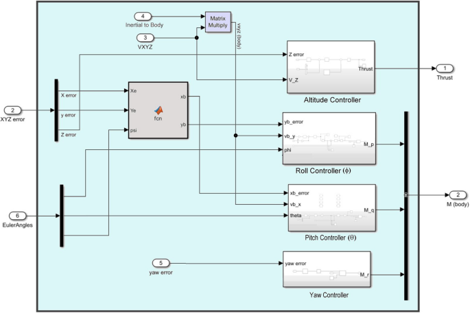
The overall Simulink model for the quadrotor incorporates a PID controller, which regulates the system by adjusting the control inputs based on the error difference between the desired and actual states
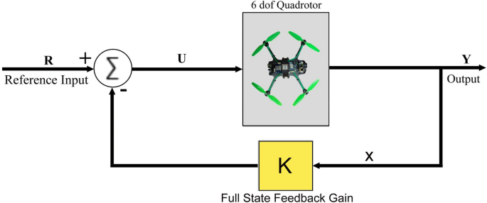
The quadrotor system operates as a closed-loop system when integrated with an LQR controller. This setup ensures that the controller continuously adjusts the system’s inputs based on feedback from the state variables, optimizing performance by minimizing the defined cost function
While the proposed hybrid PID-LQR controller demonstrates superior trajectory tracking performance, several limitations constrain its practical implementation. Dual-controller architecture increases computational complexity. The system exhibits significant sensitivity to model uncertainties, including center of gravity shifts from mounted equipment and motor parameter variations due to battery discharge or temperature changes. Additionally, in future the tuning of controllers against high-frequency disturbances common in greenhouse environments, such as sudden ventilation-induced air currents exceeding 2 m/s will be considered.
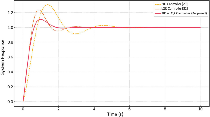
The performance of proposed controllers is evaluated and compared with state of art conventional controllers using a step response analysis


