Research on identifying damage and failure stages of backfill materials using acoustic emission data

Method overview

Classification of backfill damage and failure stages is essentially a classification problem, which can be solved through Back Propagation (BP) neural networks. This algorithm excels at modeling the nonlinear relationship between AE parameters and damage progression and leverages its adaptive learning capabilities to map complex failure mechanisms. However, the effectiveness of the model is highly dependent on the selection of discriminative input features that capture stage-specific damage signatures. Optimal feature selection reduces dimensionality, alleviates overfitting, improves interpretability, and maintains prediction accuracy.

To ensure reliable classification, AE parameters were quantitatively screened using sensitivity analysis and statistical criteria. Parameters such as energy, amplitude, and event rate were prioritized due to their strong correlation with failure stage.

Based on the selected AE parameters, a BP neural network structure is designed to accurately identify the stages of backfill damage and failure. The neural network framework includes an input layer corresponding to the selected AE parameters, a hidden layer optimized for feature extraction, and an output layer representing the classified stages of damage and failure. The specific design ensures a balance between model complexity and performance. The detailed methodology is explained as follows.

Input feature selection

The selection of input features is critical to both the efficiency and classification accuracy of the algorithm. Although principal component analysis (PCA) is widely used for dimensionality reduction, its composite projection obscures the physical interpretability of the raw parameters, and this limitation is incompatible with the goal of this study to preserve the mechanistic association between AE features and damage stages. To address this, we propose a feature selection framework based on the theoretical properties of an ideal damage-sensitive indicator. These properties include:

1. (1)

   Feature selection begins by defining an initial parameter set based on traditional AE parameters. In this study, time-domain parameters such as rise time, ringdown number, energy, duration, amplitude, and absolute energy were selected as basic metrics. To enrich this dataset, frequency domain characteristics were derived by applying Fourier transform analysis to the raw AE waveforms and extracting the dominant frequencies of each signal. These parameters collectively form an initial indicator set φ = {rise time, number of calls, energy, duration, amplitude, absolute energy, dominant frequency}.

2. (2)

   To reduce stage boundary ambiguity during damage stage delimitation, data sampling intervals should be chosen strategically to exclude transition zones where signal overlap may distort parameter sensitivity. In this study, we adopt a moving window algorithm to define a stable interval of feature extraction controlled by the following criteria:

   $$\left\{ {\begin{array}{*{20}l} {F = a + \left( {b – a} \right)/3} \hfill \\ {E = b – \left( {b – a} \right)/3} \hfill \\ \end{array} } \right.$$

   (1)

   where F represents the start time of the extraction, E Indicates the end time of the extraction. be indicates the start time of the stage, b represents the end time of the stage.

3. (3)

   Metrics with robust representativeness exhibit two important properties: low variability within individual stages and high variability between individual stages. To quantify these properties, principles of mathematical statistics with variance are applied. \(\left( {D_{i,j} \;\left( {i = 1,2, \ldots ,4\;j = 1,2, \ldots ,7} \right)} \right)\) Measuring intra-stage variability and mean values \(\left( {E_{i,j} \;\left( {i = 1,2, \ldots ,4\;j = 1,2, \ldots ,7} \right)} \right)\) Evaluate differences between stages. here, I indicates the stage number, j corresponds to the indicator index in the acoustic emission dataset φ defined in step (1).

4. (4)

   To assess the representativeness of the indicators, the average within-stage variance (P_I), quantifying stability by measuring the within-stage mean variation and between-stage mean variance (Q_I), which captures discernment through branching between stages. Very representative indicators are kept to a minimum P_I (low intra-stage variation) and maximize Q_I (significant differentiation between stages), ensuring both stability over repeated observations and sensitivity to different operating conditions.

5. (5)

   To ensure scale invariance, the average within-stage variance (P_I) and the variance of the interstage mean (Q_I) is normalized by min-max scaling to obtain dimensionless values. P_I' and Q_I“Within range” [0, 1]. Sensitivity factor \(\alpha_{i}\) Then, is defined as the ratio of normalized discriminative power to stability.

   $$\alpha_{i} = \frac{{Q_{i}^{\prime } }}{{P_{i}^{\prime } }}$$

   (2)

6. (6)

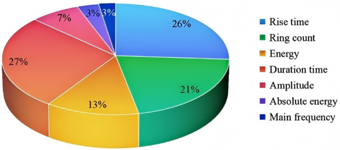
   To rigorously assess the importance of an indicator, the contribution vector βderived from the sensitivity coefficient \(\alpha_{i}\) Through equation (3), we quantify the relative discrimination weight of each indicator. A statistical significance test with a 5% threshold is applied, as shown in Figure 3. βexclude unimportant metrics. This process identifies five statistically significant features (rise time, number of calls, energy, duration, amplitude}) as the optimal inputs to the neural network, ensuring dimensionality reduction while preserving diagnostically relevant signal properties.

   $$\beta_{i} = \frac{{\alpha_{i} }}{{sum\left( {\alpha_{i} } \right)}}$$

   (3)

Designing the BP Neural Network Classification Algorithm

Data extraction for neural network input and output layers

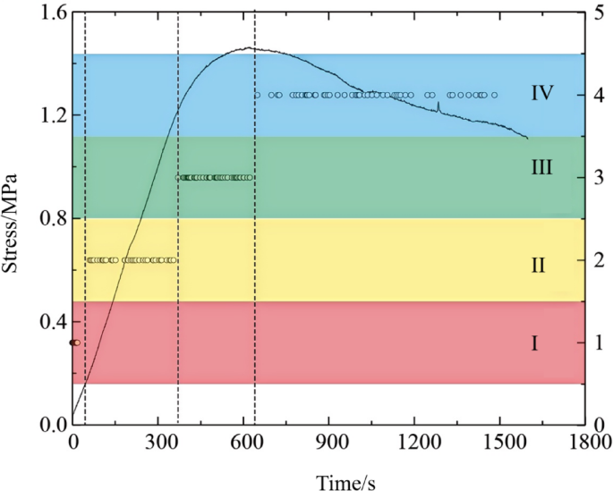
Backpropagation (BP) neural networks are very suitable for classifying damage and failure stages in backfill materials because they can autonomously learn the nonlinear relationship between input features and target outputs. This study utilizes the AE parameters {rise time, number of calls, energy, duration, amplitude} as input features. These parameters are normalized to eliminate scale mismatches and input into a network architecture designed to map the AE signature to four damage stages (initial compression stage, elastic stage, yield stage, and post-peak failure stage) derived from the stress-time curve. The output layer consists of four nodes, each of which produces a value between 0 and 1 representing the probability of the input belonging to its respective damage stage. The classification of samples in the dataset into these four stages follows the definitions shown in Table 1.

To ensure unbiased model generalization, the experimental data were partitioned using a stratified random sampling approach to maintain a proportional representation of each damage stage (initial compression, elastic, yield, and post-peak failure) in both the training and validation sets. From the complete dataset, 80% samples were allocated for training and 20% independent samples were reserved for validation, and typical training data for each damage stage is shown in Table 2. This approach reduces overfitting to stage-specific anomalies and ensures that the model learns robust patterns across all stages of deformation. Using monitoring data from a representative specimen as an example, Figure 4 shows the distribution of training and validation data across all injury stages, confirming the balanced coverage of each stage.

BP neural network architecture design

The BP neural network in this study uses two hidden layers to model the nonlinear relationship between AE parameters and backfill damage stage. The input layer consists of five nodes, each corresponding to an AE parameter (rise time, ring count rate, energy, duration, amplitude), and the output layer consists of four nodes representing damage stages (Table 1). A softmax activation function is applied to the output layer to generate mutually exclusive probabilistic outputs, and the final classification is determined by selecting the stage exhibiting the highest probability value.

It is important to determine the optimal number of hidden layer nodes. Too few nodes limits the network's ability to capture nonlinear patterns, reducing accuracy. On the other hand, too many nodes increases computational complexity and the risk of overfitting, thereby reducing generalizability.

The empirical formula (Equation 4) guides the initial node selection.

where I is the number of hidden layer nodes. n represents the number of input layer nodes (in this study, n = 5), and metersis the number of output layer nodes (in this study, meters= 4). Therefore, the number of nodes in the hidden layer was set to 7 to balance model complexity and computational efficiency.

The final architecture consists of an input layer (5 nodes), two hidden layers (7 nodes each with ReLU activations), and an output layer (4 nodes with softmax activations). Dropout regularization (rate = 0.2) is incorporated between layers to enhance generalization, and training is performed using categorical cross-entropy loss for stochastic optimization.