This paper uses a published planetary gearbox dataset as source data.30. The failed planetary wheel is used to replace the original normal planetary wheel in simulation experiments. Vibration data is collected by a Sinocera CA-YD-1181 accelerometer. All channels have sample rates set to 48 kHz. The detailed parameters of the planetary gearbox and the relationship between the two important fault-related frequencies and the input shaft frequency are shown in Table 3.
In this study, we test the performance of the proposed method on PCNN + EEMD + GADF + SPKO using only the first channel of the planetary gearbox vibration signal. Vibration signals five states of five states, including health, broken teeth, wear gear, cracks, missing teeth, etc., as inputs to this model, and classification as outputs. The diagnostic process for planetary gearbox tomography signals is shown in Figure 4.
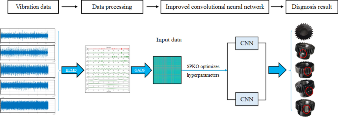
Planetary gearbox fault signal diagnosis.
CNN input processing based on EEMD and GADF
The dataset contains five types of vibration signals: health, tooth fractures, wear gear, cracks, missing teeth. The EEMD method is used for signal decomposition. Broken tooth faults and crack faults were taken as case studies and the results of the decomposition of these two fault types using EEMD technology are shown in Figure 5.
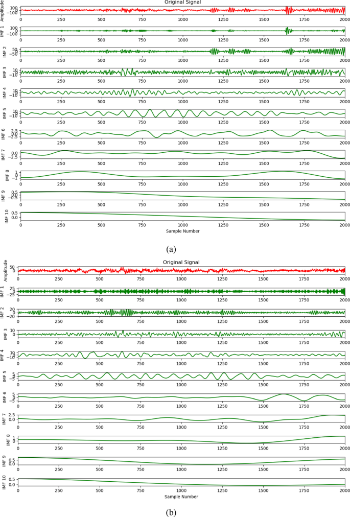
EEMD decomposition results of broken tooth faults (a) and cracked faults (b).
As seen in Figure 2. 5 and 10 IMF31 Different periods are generated. Most of the IMF components have been found to be steady signals, oscilling the zero average. EEMD efficiently converts nonlinear series into multiple steady-state time series. Converting the above processing tomographic signals as input to the CNN into a GADF image will retain all the fault information and maintain connections between the signals at different time intervals. Therefore, GADF is suitable for processing planetary gearbox fault vibration signals with time-varying characteristics. 2000 sampling points are used as one sample to ensure that all vibration samples collected by the vibration sensor contain at least one complete fault cycle. After GADF treatment, fault signals obtained in five conditions: health, teeth, wear gear, cracks, and tooth missing as shown in Figure 6. Each category has 3000 samples.
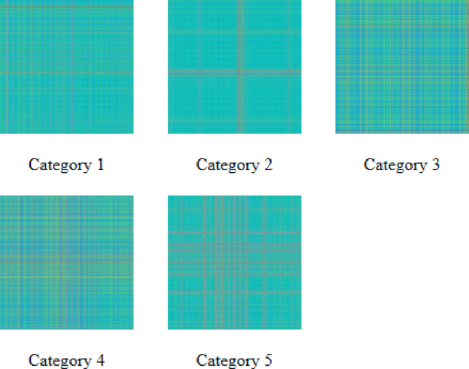
Category 5 fault signal GADF diagram.
Vibration signals are processed using EEMD and GADF methods and entered into the CNN model to compare the accuracy of fault diagnosis. The comparison results are shown in Figure 7.
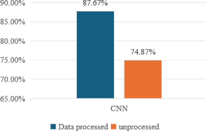
Comparison of diagnostic accuracy with or without data processing.
As seen in Figure 7, the vibration signal is decomposed using the EEMD method and converted to a 2D image using the GADF method. The raw signals are processed to improve the accuracy of fault diagnosis and demonstrate the effectiveness of the methods proposed in the section. 4.
Fault prediction results for multilayer CNNs
Comparative experiments containing the same proportion of samples
Each type of failure data has 3000 samples, with 70% of the data segment being randomly selected as the training data set, and the other 30% being used for testing. To ensure the accuracy of the experiment, each set of experiments is repeated over 5 rounds and the final results are averaged. Results are shown in Table 4, with the best results marked in bold.
From Table 4, we can see that the CNN model has a low diagnostic performance of only 87.21%. The PCNN diagnostic results were 90.88%, which is higher than the CNN model. It shows that parallel structures improve diagnostic accuracy. The confusion matrix of the test set of CNN and PCNN models with diagnostic accuracy is shown in Figures 2 and 2. 8 and 9.
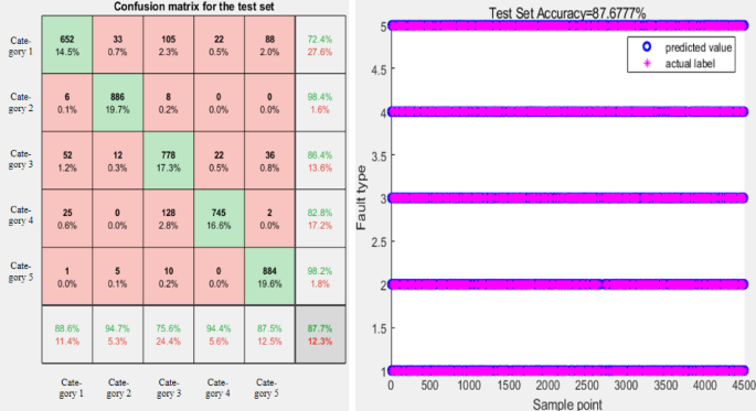
CNN model tests set the confusion matrix and diagnostic accuracy.
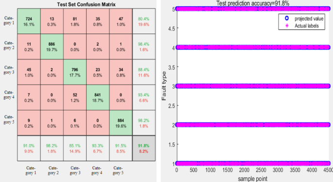
PCNN model tests set the confusion matrix and diagnostic accuracy.
To observe whether the PCNN model is overfitted, we use the learning curve.32 It should be analyzed as shown in Figure 10.
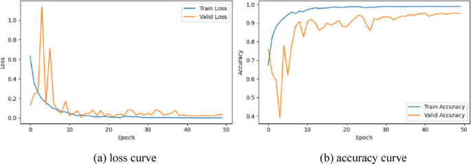
Loss and accuracy curves for PCNN models.
As can be seen in Figure 10, after 30 iterations, both the loss function and the accuracy curve converge to the region. The loss function value is approximately 0.04. The accuracy is approximately 91%. There is no overfitting.
Comparative experiments using different proportions of samples
To test the universality of the method in this paper, experiments are carried out at various proportions of data samples. Sampled at 4:2:2:1:1 depending on the frequency of failures of different types of gearboxes. The experimental data set is divided into 3,000 groups in normal state, 1,500 groups in broken teeth, 1,500 groups in worn state, 750 groups in cracked state, and 750 groups in missing teeth. The training and test sets are randomly divided into 7:3 ratios. To avoid experimental chances, each group repeats the experiment five times before average. The diagnosis results are shown in Table 5.
As shown in Table 5, the diagnostic accuracy of the PCNN model is 85.68%, an improvement of about 4% compared to CNN. At different sample ratios, multi-layered convolutional neural networks exhibit better performance than traditional convolutional neural networks. The confusion matrix and diagnostic accuracy of the test sets of CNN and PCNN models are shown in Figures 2 and 2. 11 and 12. To further improve the accuracy and robustness of planetary gearbox fault identification, we use the SPKO algorithm to improve and optimize hyperparameters in PCNN models.
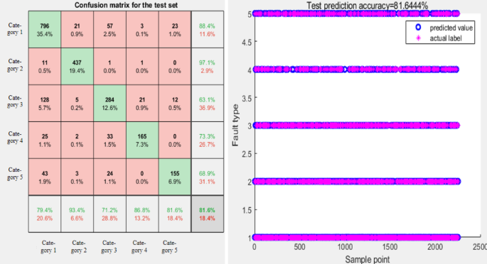
CNN model tests set the confusion matrix and diagnostic accuracy.
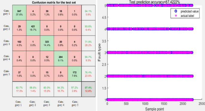
PCNN model tests set the confusion matrix and diagnostic accuracy.
To observe whether the PCNN model is overfitting under unbalanced data, the learning curve should be analyzed, as shown in Figure 13.
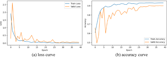
Loss and accuracy curves for PCNN models.
As can be seen in Figure 13, after 30 iterations, both the loss function and the accuracy curve converge to the region. The loss function value is approximately 0.07. The accuracy is approximately 86%. There is no overfitting.
Model optimization based on SPKO algorithm
The initial parameters for the PKO and SPKO algorithms are set with the overall size 3 and the maximum number of loop iterations. This is used to optimize hyperparameters, training rate, batch size, and L2 normalization coefficients in convolutional neural network models. The experiments are then performed at different rates of 7,500 samples, with the same percentage as 15,000 samples each. The training and test sets are randomly divided into 7:3 ratios. To avoid experimental chances, each set is averaged after five repeated experiments. Final diagnostic results were obtained as shown in Table 6, with optimal results marked in bold.
The proposed method using a balanced sample The diagnostic accuracy of SPKO-PCNN is 95.94%, which is higher than that of the PKO-PCNN model. SPKO-PCNN has over 85% diagnostic accuracy for different proportions of samples. SPKO-PCNN shows that failures can be diagnosed in cases of lack of data samples and imbalances for reducing data samples. At the same time, the SPKO algorithm is used to learn model parameters, and due to the robustness of the SPKO algorithm itself, the variability in the accuracy of fault recognition is relatively small. The SPKO-PCNN model was used to diagnose samples of the same percentage, and results are compared with previous studies, as shown in Figure 14.
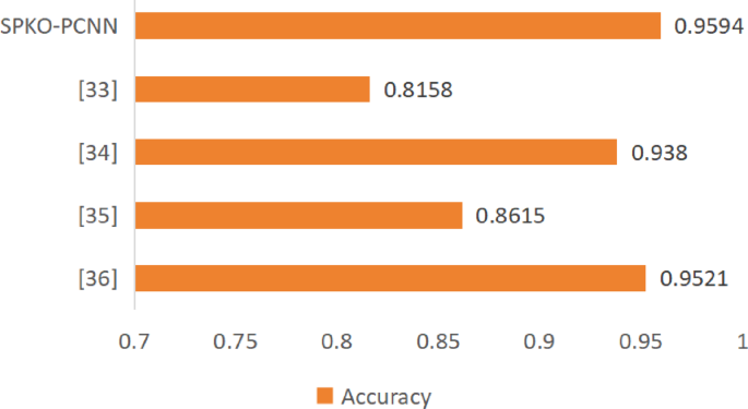
Comparison results with other studies.
As can be seen in Figure 14, the diagnostic accuracy of the SPKO-PCNN model is higher than that of the literature33,34,35,36. The SPKO-PCNN method employed in this paper can effectively improve the accuracy of planetary gearbox fault identification. Meets the requirements for fault diagnosis in real-world applications.


