The findings of this study reinforce and extend the conclusions of prior research in soil temperature modeling. For instance, Citakoglu18 demonstrated that ANFIS and ANN models outperform classical statistical methods for ST estimation. Building on this, our results show that the ANN model achieved a superior correlation coefficient (r = 0.98) and reduced RMSE values, particularly at depths of 50 cm and 100 cm, compared to SARIMA and MLR models. Similarly, while Feng et al.3 identified ELM as the most effective method, our ANN approach demonstrates higher adaptability and accuracy under the unique meteorological conditions of Riley Station.
This study also highlights the influence of meteorological parameters, with surface temperature (Avg. Infrared) and air temperature (Avg. T) identified as the most critical variables for accurate ST prediction. These findings align with Sattari et al.6, emphasizing air temperature’s importance in their predictive models. Significantly, our work extends these insights by quantitatively demonstrating how the ANN model outperforms other machine-learning techniques in capturing non-linear and depth-dependent variations in ST.
These results validate the applicability of ANN models for complex ST prediction tasks and highlight their practical benefits in agricultural management. The ANN model’s ability to accurately predict ST with minimal input parameters suggests a transformative potential for field applications, enabling cost and time efficiency. By advancing the understanding of model performance across depths and conditions, this research establishes a benchmark for future studies in soil temperature modeling.
Modeling results
Identifying whether the data has a specific correlation due to seasonal fluctuations is critical. For this reason, input data for 2020 and 2021 were categorized into hot and cold seasons, and then correlation analysis was done independently for each season. To investigate the distribution characteristics of ST at different depths, descriptive statistical indices such as mean, standard deviation, minimum, maximum, skewness and kurtosis were calculated (Table 5).
The results show that the average ST has a relatively stable trend with increasing depth, but the value of the standard deviation at some depths shows changes that indicate temperature fluctuations in these layers. Skewness values are close to zero in most depths, which indicates a relatively symmetrical distribution of data. However, at the depths of 10, 20 and 100 cm, negative skewness is observed, which indicates the skewness of the data distribution towards values lower than the mean. On the other hand, Kurtosis values are negative in all depths, which indicates that the data distribution is wider and has shorter tails than the normal distribution. These patterns indicate the relative stability of temperature in different soil depths as well as the possible influence of environmental and seasonal conditions on temperature variability.
Figure 5 (a to c) shows the scatterplot matrix for two seasons, i.e., hot and cold. The matrix comprehensively shows the correlations between dependent and independent variables. Data from January, February, March, October, November, and December were used for the cold season. For the hot season, data from the other months, April, May, June, July, August, and September, were utilized as input in the correlation study. The results reveal that seasonal fluctuation has little influence on soil temperature at various depths Fig. 5 (a and b). As a result, it was determined that separating the data would be ineffective. As a result, the association between the parameters was discovered utilizing the whole daily data set for 2020 and 2021. Figure 5 (c) shows independent factors and correlation values that greatly influence daily ST. When measuring soil temperatures at depths of 5, 10, and 20, it was found that the surface (skin) temperature (Avg. Infrared) was the most significant meteorological variable, while air temperature (Avg. T) was substantial at depths of 50 and 100 cm.
The analysis revealed that the influence of meteorological parameters on ST varies significantly with depth. At shallower depths of 5, 10, and 20 cm, the surface (skin) temperature, represented by the average infrared (Avg. Infrared) parameter, emerged as the most significant variable. This can be attributed to the direct and immediate effect of surface radiation and heat transfer on the upper soil layers, where thermal energy from the surface penetrates without substantial attenuation. As a result, fluctuations in surface temperature are strongly correlated with ST at these depths.
In contrast, at deeper soil layers (50 and 100 cm), air temperature (Avg. T) became the dominant influencing factor. This shift is likely due to the diminished direct impact of surface radiation as thermal energy dissipates while moving downward through the soil. At these depths, heat transfer processes, such as conduction, rely more on the ambient air temperature, which exerts a more consistent and long-term influence. These findings align with the principles of thermal conductivity in soils, where heat transfer at greater depths is slower and primarily influenced by stable external factors like air temperature.
The distinct differences in the significant predictors across soil depths highlight the importance of considering depth-specific meteorological parameters in soil temperature modeling. This insight also reinforces the need for tailored predictive models that account for varying physical and thermal dynamics at different soil layers.
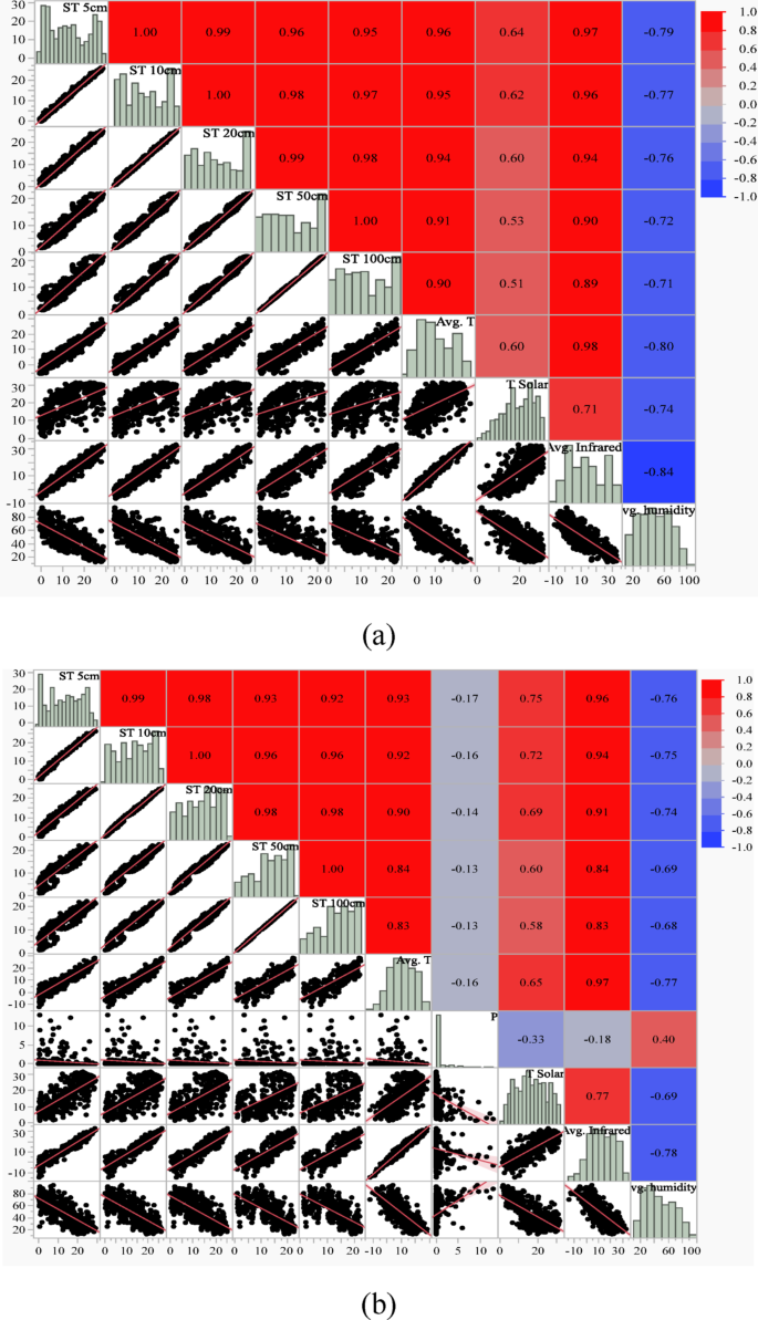
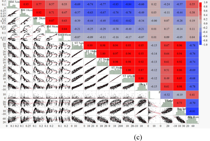
Correlation coefficient scatterplots of soil temperature (ST) at various depths (5, 10, 20, 50, and 100 cm) with meteorological parameters: average temperature (Avg. T), precipitation (P), solar radiation (T Solar), surface temperature (Avg. Infrared), and humidity (Avg. Humidity). The plots represent data for (a) hot seasons, (b) cold seasons, and (c) the combined daily dataset from 2020 to 2021.
Based on the analyses, SARIMA was deemed appropriate for the forward prediction of daily ST data with the indicated seasonality pattern. The SARIMA model results are given in Table 6. The SARIMA model was built using daily data from 2020 to 2021. The model’s effectiveness was evaluated using data collected in 2022.
The orthogonal least squares estimation approach was used to investigate the importance of input variables in predicting daily ST at different depths15. An absolute value Pareto plot of the estimates is included in the Fit Last Squares Pareto plot report40. The order of model term entry affects the orthogonal estimates. Estimates are transformed into orthogonal forms and standardized for equal variances. The importance of input variables in predicting daily ST for different depths is presented in Tables 7, 8, 9, 10 and 11; Fig. 6 (a-e). Average air temperature (Avg. T), solar radiation (T Solar), surface temperature (Avg. Infrared), and relative humidity (Avg. Humidity) are the essential meteorological variables in daily ST prediction.
In comparison, precipitation (P) has the most negligible significance on daily ST. In addition, the effect of precipitation on soil temperature is insignificant in all models and different soil depths. As a result, the precipitation parameter was ignored in the used models.
In Fig. 6 (a-e), Pareto charts showing the importance of meteorological parameters used in estimating daily soil temperature at different soil depths (5 cm, 10 cm, 20 cm, 50 cm and 100 cm) are presented, and these charts were constructed using the orthogonal least squares method in order to determine the essential meteorological parameters for each depth; in the charts, the effect of the parameters on the estimation is expressed by the “Orthog t-Ratio” values and the parameters with the highest values stand out as the most important factors; while the surface temperature (Avg. Infrared) is the most critical parameter at the depths of 5 cm, 10 cm and 20 cm, the air temperature (Avg. T) plays a more decisive role at the depths of 50 cm and 100 cm; also the effect of other parameters such as solar radiation (T Solar) and humidity (Avg. Humidity) remains at lower levels, while precipitation (P) is observed to be the parameter with the least effect at all depths.

(a–e) Pareto plot of orthogonal estimates (a) ST 5 cm, (b) ST 10 cm, (c) ST 20 cm, (d) ST 50 cm, (e) ST 100 cm.
The results determined that surface temperature (Avg. Infrared) is the most essential meteorological variable in estimating daily ST at 5, 10, and 20 cm depths. In comparison, air temperature (Avg. T) is the most effective meteorological parameter in assessing daily ST at 50 cm and 100 cm depths. In a similar study, Sattari et al.6 stated that air temperature is the most critical parameter in predicting ST, which is consistent with the results of the present study. The difference in the importance of parameters is probably related to the complex simulation process and non-linear mathematical relationships between independent and dependent variables in different predicting models41.
Figure 7 shows the daily soil temperature (ST) estimates of the SARIMA model at different soil depths (5 cm, 10 cm, 20 cm, 50 cm and 100 cm) within a 95% confidence interval. SARIMA captures seasonal fluctuations and trends, especially at near-surface depths (5 cm, 10 cm, 20 cm). A strong agreement is observed between the model’s estimates and the actual values at these depths. However, the model performs relatively poorly at deep soil layers (50 cm, 100 cm). This is because temperature changes in deep soil layers are slower and more complex. Although SARIMA effectively captures seasonal and short-term trends, it may be limited in modeling long-term dynamics in deep soil layers. Therefore, it is recommended that more advanced models (e.g. ANN) be used in deep soil layers. The SARIMA model provides reliable estimates, especially in near-surface soil layers, which provides a significant advantage in agricultural applications. A potent tool is time series forecasting with the most minor inaccuracy. The components are split into systematic and non-systematic components to help pick forecasting methods for time series. Non-systematic components cannot be directly modeled, whereas systematic components are recognizable, regularly repeating components. Trend and seasonality are categorized as systematic components, whereas noise is non-systematic42.
(a–e) Estimation of ST by SARIMA model for different depths (a) 5 cm, (b) 10 cm, (c) 20 cm, (d) 50 cm, and (e) 100 cm.
Table 12 displays the models developed using MLR analysis and least square Estimation prediction expressions. In addition, the predicted daily ST values by the models and the observed values are compared in Fig. 8 for different depths. The residual diagrams of the studied models are shown in Fig. 9.
Figure 8 shows that the ANN model performs better than the SARIMA and MLR models at different soil depths. These findings support that the ANN model is the most effective for predicting soil temperature. Furthermore, the graph’s deviations and errors reveal the models’ limitations and areas for improvement.
SARIMA Model: The estimates based on time series analysis successfully captured the seasonal fluctuations, especially at the near-surface depths (5 cm, 10 cm, 20 cm). However, more significant deviations were observed in the estimates at the deep soil layers (50 cm, 100 cm). This is due to the more complex temperature dynamics in the deep layers.
MLR Model: The estimates based on linear regression showed an acceptable performance, especially at the near-surface depths. However, since it could not capture non-linear relationships, the prediction errors increased in deep soil layers. This reveals the limitations of the MLR model.
ANN Model: The artificial neural network model agrees with actual observations at all depths. In particular, its ability to capture complex and non-linear relationships provided more accurate predictions in near-surface and deep soil layers. This proves the superior performance of the ANN model.
Near-Surface Depths (5 cm, 10 cm, 20 cm): All models performed relatively well in near-surface layers. However, the ANN model had the lowest error margin and the highest prediction correlation.
Deep Soil Layers (50 cm, 100 cm): While the prediction performance of the SARIMA and MLR models decreased in deep layers, the ANN model showed a consistent performance. This indicates that ANN can better model the complex temperature dynamics in deep layers.
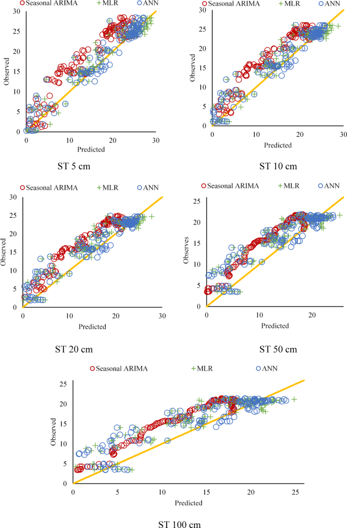
Estimation of ST by SARIMA, MLR, and ANN models for different depths.
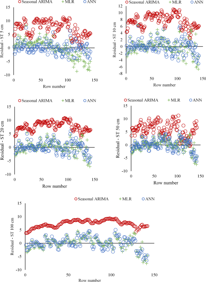
Residual plots for SARIMA, MLR, and ANN models for different depths.
The comparison of different machine learning algorithms for all soil depths shows the high capability of proposed models in predicting daily ST. The ANN model offers a more reliable statistical relationship based on the calculated statistical indicators than other models.
The regression coefficients express a favorable fit between the observed and the predicted values by the ANN model. The most suitable model fitted in 5 cm to 100 cm soil layers is related to the ANN model. The acceptable performance of the ANN model has also been reported in the study of other researchers, which is consistent with the results of the present study23,43,44,45. The MLR and SARIMA models performed less than the ANN model based on the evaluation criteria values. However, MLR and SARIMA models have acceptable predictions of daily ST, which can help estimate daily ST in the impossibility of using the ANN model. According to Khan et al.46, ANNs are a fresh subset of soft computing with a wide range of applications. It is, therefore, possible to categorize or forecast future values using the ANN model.
The performance of neural network models is not required in simple operations; the goal is to use them in models requiring intensive calculations. It has been effectively used in numerous fields because of its fault tolerance. It is applied in fields including categorization, image recognition and optimization, handwriting recognition, churn analysis, meteorological forecast, and soil property prediction to achieve high application performance46,47. Artificial neural networks (ANNs) can detect complex temporal variations46. For rapid, low-data requirements, ANN offers the advantage of a data-driven, functional, and user-friendly approach48. The results of predicting models show that daily ST estimation based on meteorological data decreases with increasing soil depth. The effect of soil moisture on heat transfer in the soil is one of the main reasons for this problem. Several studies have reached similar results, which agree with the present study’s results18,23,49,50. Data mining models perform better monthly ST estimation at 5 and 10-cm soil depths3,8,51. Yusefi et al.52 similarly found that ST decreased with increasing depth, and the correlation between ST and meteorological parameters decreased.
Figure 10 clearly shows that the ANN model is superior to other models in soil temperature prediction. Taylor diagrams are an effective tool for visually comparing the performance of models, and in this study, the ANN model stands out with higher accuracy and lower error rates. These findings support the idea that the ANN model can be a reliable tool for soil temperature prediction in agricultural and environmental applications. The results show that the ANN model with r = 0.98 outperforms the SARIMA and MLR models in forecasting future daily ST at different depths. The highest and lowest determination coefficients between daily ST and meteorological parameters are related to 5–20 cm depths. The results showed that these coefficients decrease with increasing soil depth. The results of the studies of Tabari et al.5 and Citakoglu18 are based on the accuracy of ANN in predicting ST compared to other data mining methods, which agrees with the results of the present study.

(a–e) Taylor diagrams of the SARIMA, MLR, and ANN models for different depths (a) 5 cm; (b) 10 cm; (c) 20 cm; (d) 50 cm; (e) 100 cm.
Table 13 shows the performance comparison of implemented Models for Training and Testing Datasets. A comparative box plot and a radar chart (Figs. 11 and 12) are included to show the distribution of model predictions at different soil depths. These visualizations provide a more explicit representation of changes in model performance. ANN model offers the most accurate and reliable forecasts of daily ST, outperforming both the SARIMA and MLR models. This underscores the potential of ANN to capture complex, non-linear relationships between soil temperature and various meteorological parameters.
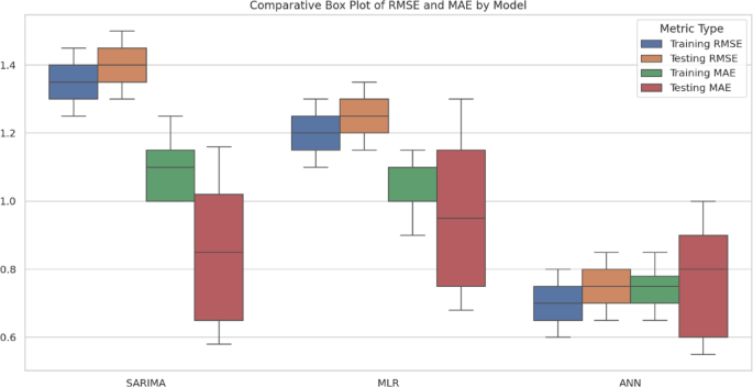
Comparative Box Plot of RMSE and MAE for all models.

Comparative radar chart of RMSE and MAE for all models and soil depths.
Comparison with similar investigations
The statistical criteria values for five intelligent methods, including the ANFIS model18, decision tree (DT) and gradient boosted trees (GBT)41, ELM, and generalized regression neural networks (GRNN)3 are shown in Fig. 13. The data presented in Fig. 13 were sourced from prior studies that evaluated the performance of intelligent methods for soil temperature prediction under similar conditions. Performance metrics, including RMSE and r values, were extracted from the referenced literature3,18,41. These values were normalized where necessary to ensure consistency in evaluation criteria and enable a direct comparison with the present study. The metrics for the ANN model proposed in this study were calculated based on experimental results obtained using the same dataset and validation methods. This comparative analysis highlights the superior performance of the ANN model, particularly in achieving lower RMSE and higher correlation coefficients (r) compared to the alternative methods.
According to the evaluation criteria results, the ANN technique is within a more appropriate and acceptable error range for estimating daily ST than other intelligent methods. Furthermore, the ANN method has adequate power to distinguish between various daily ST levels. Compared to other methods, ANN performed well under nearly identical circumstances. Applying the proper parameters allows ANN to predict daily ST with reasonable accuracy. Although having more input parameters available yields more accurate solutions, intelligent models’ ability to adapt to input data makes it possible to pick the best available options while still getting the outcomes you want. ANFIS, DT, GBT, ELM, and GRNN all improved in determination coefficient criteria by 1–2%, respectively. The best method for estimating daily ST can be generally introduced as an intelligent strategies. The high accuracy of the ANN can lead to an accurate estimation of ST in different regions based on the data available in other stations. The advantage of the ANN is that its estimated results are close to the actual field conditions. The analysis considers ST levels at different soil depths in ANN. Also, ANN can provide an appropriate estimation of ST by only having soil temperature values in various soil layers, which reduces calculation time for moving applications. In general, it is suggested to work on the real-time applications of the ANN model and measure other soil conditions, such as the amount of salt and other elements present on its accuracy. The performance obtained by the ANN model is far from the ideal state, and there is room for more improvement in the field.
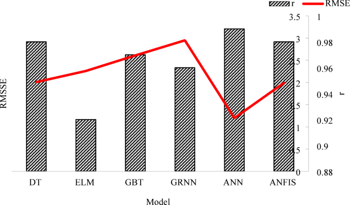
Comparison of intelligent prediction methods for soil temperature (ST) using RMSE and correlation coefficient (r). Data for ANFIS, Decision Tree (DT), Gradient Boosted Trees (GBT), Extreme Learning Machines (ELM), and Generalized Regression Neural Networks (GRNN) were sourced from previous studies3,6,18 and normalized for consistent evaluation with the ANN model developed in this study.
The findings of this study underline the critical importance of accurate soil temperature (ST) prediction for agricultural and environmental management. By addressing the limitations of direct ST measurements, such as high costs and limited synoptic station coverage, this research demonstrates the efficacy of data-driven models in filling these gaps.
Among the models evaluated, the Artificial Neural Network (ANN) model stands out for its superior performance in predicting ST at multiple depths. The ANN’s ability to capture complex non-linear interactions between meteorological parameters and ST highlights its robustness and adaptability compared to traditional methods like Multiple Linear Regression (MLR) and Seasonal ARIMA (SARIMA). This study’s application of ANN to soil temperature modeling represents a significant advancement, notably as it demonstrates the model’s ability to generalize across varying soil depths with minimal error, as evidenced by its high correlation coefficient (r = 0.98) and low RMSE values.
The findings also highlight the depth-specific influence of meteorological parameters on ST, with surface temperature (Avg. Infrared) playing a dominant role at shallow depths (5, 10, and 20 cm), while air temperature (Avg. T) becomes the key predictor at deeper levels (50 and 100 cm). These insights provide a deeper understanding of the thermal dynamics within soil profiles, which is crucial for optimizing agricultural practices such as irrigation scheduling, crop management, and climate-resilient farming.
Furthermore, the comparative analysis with other intelligent prediction methods, such as ANFIS, Decision Trees, and gradient-boosted trees, underscores the ANN model’s ability to outperform these alternatives under similar conditions. This comparative framework validates the methodological approach adopted in this study and provides a benchmark for future research in soil temperature modeling.
In summary, this research substantially contributes to the field by offering a scalable, efficient, and accurate framework for soil temperature prediction. Integrating advanced machine learning techniques with real-world meteorological data bridges the gap between theoretical advancements and practical applications, providing actionable insights for sustainable agricultural and environmental management.
Advantages and limitations of the proposed model
The proposed ANN model has shown high prediction accuracy (r = 0.98 and low RMSE values) at different soil depths (5 cm, 10 cm, 20 cm, 50 cm and 100 cm) and can successfully capture the complex, non-linear relationships between soil temperature and meteorological parameters. This provides a significant advantage in an area where traditional models (e.g., MLR and SARIMA) are limited. The model has yielded practical results both near the surface and in deep soil layers, and its ability to predict soil temperature using only meteorological data offers a great advantage, especially in cases where measurements are costly and time-consuming. In addition, its easy adaptability to different geographical regions and climatic conditions allows the model to have a wide range of applications. However, the model has some limitations. The ANN model requires a large amount of high-quality data for training, and its performance may deteriorate if the data set is limited or noisy. The complex structure of the model and the long training process may increase the computational cost, especially in large data sets. In addition, the lower performance in deep soil layers (50 cm and 100 cm) compared to near-surface layers is due to the more complex temperature dynamics in these layers. The fact that the model is considered a “black box” and its internal workings are challenging to interpret may be a limitation for users, especially in agricultural applications. Finally, the model depends on meteorological data; if these data are missing or incorrect, the forecast performance may be negatively affected.


