
Data initialization
The dataset of 191 HPC mixtures, collected from38, required preprocessing to ensure data quality and consistency. Missing values, present in less than 5% of the entries (mainly for superplasticizer and fly ash), were imputed using median values to maintain statistical distributions, as the calculated mean can be skewed by outliers. Outliers, identified using the interquartile range (IQR) method (values beyond 1.5 × IQR), were identified in water-to-binder (W/B) and silica fume (SF) ratios for approximately 3% of the samples and were removed to avoid model bias. Inconsistencies, such as non-standard units for CS or slump flow, were reconciled by converting all measurements to MPa and mm, respectively, in accordance with ASTM standards. Feature standardization (zero mean, unity variance) was applied to normalize the input ranges and increased the convergence of the model during training (Table 1).
The assessment of slump Strength characteristics for high-performance concrete samples was conducted after 28 days. Additionally, a grain size of 7.2 and a specific density of 2.7 for coarse aggregates derived from crushed granite measuring 19 mm were utilized in the studies. Portland cement was chosen in accordance with ASTM standard Type I. Naphthalene-based superplasticizer was utilized to diminish water content and regulate the water-to-binder ratio. It is important to remember that aggregates consist of fine silica sand with a specific gravity of 2.61 and a fineness coefficient of 2.94. Table 2 shows the target values of the training section and the statistical characteristics of the input of the proposed model. The slump test conformed to ASTM C 143-90a standards following quick mixing in accordance with ASTM C 231-91b guidelines.
Figure 2 illustrates the relationships between the ingredients and the Strength characteristics of concrete samples. Furthermore, the heat maps in Fig. 3 illustrate the simultaneous impact of the water content variable (W) in conjunction with W/B, S/A, and SF on the slump and CS of HPC samples. The significant correlation coefficients between Strength parameters and HPC components are linked to silica fume and superplasticizer, exhibiting correlation values between 0.8 and 1 for CS and between 0.2 and 0.4 for slump.

The values indicating the relationship between HPC components and Strength characteristics.

T-S fuzzy inference system (T-SFIS)
The T-SFIS network structure has two phases called the result and the hypothesis part. Training T-SFIS indicates specifying the parameters related to these phases. T-SFIS uses existing inputs to output data pairs during training. Then can obtain the IF–THEN fuzzy rules that connect these phases40. As shown in Fig. 3, the T-SFIS structure contains 5 layers. T-SFIS has a Two-input, one-output structure and 4 rules. Hierarchical structure of T-SFIS is defined below.
-
a)
Layer one
The first layer is referred to as the Fuzzification Layer. A fuzzification layer employs membership functions to derive fuzzy sets from input data. The parameters that define the format and membership functions are referred to as prerequisite parameters, with {a, b, c} representing the necessary parameter locations41. The membership degree is computed for each membership function by applying these parameters in Eqs. (1) and (2). The membership degrees acquired from this stratum are represented by \({\delta }_{x}\) and \({\delta }_{y}\):
$${\delta }_{{A}_{i}}\left(x\right)=gbellmf\left(x;a,b,c\right)=\frac{1}{1+{\left|\frac{x-c}{a}\right|}^{2b}}$$
(1)
$${U}_{i}^{1}={\delta }_{{A}_{i}}\left(x\right)$$
(2)
-
b)
Layer two
The dominant layer is referred to as layer two. The fuzzy layer employs the computed membership values to provide rule trigger intensities (vi)42. Reinforcement learning approaches for nonlinear systems42 complement metaheuristic algorithms like GWO and QPSO in optimizing HPC prediction models. The vi value is calculated by multiplying the membership values as indicated in Eq. (3):
$${U}_{i}^{2}={v}_{i}={\delta }_{{A}_{i}}\left(x\right).{\delta }_{{B}_{i}}\left(y\right) i=\text{1,2}.$$
(3)
-
c)
Layer three
The normalizing level designates layer three. Determine the normalized firepower corresponding to each rule. Moreover, the normalized value represents the ratio of the fire intensity of the ith rule to the total sum of all fire intensities, expressed as:
$${U}_{i}^{3}={w}_{i}=\frac{{v}_{i}}{{v}_{1}+{v}_{2}+{v}_{3}+{v}_{4}} i\in \{1, 2, 3, 4\}$$
(4)
-
d)
Layer four
Defuzzification Layer is the designation for layer four. Fuzzy-based control methods, such as those for multi-agent systems43, support the application of T-SFIS in modeling HPC properties. A weighted rule value is computed for each node in this layer. This value is ascertained utilizing a first-order polynomial in Eq. (5):
$${U}_{i}^{4}={w}_{i}{f}_{i}={w}_{i}({q}_{i}x+{p}_{i}y+{r}_{i})$$
(5)
where {\({q}_{i}\), \({p}_{i}\), \({r}_{i}\)} denotes the parameter set and \({w}_{i}\) denotes the normalization layer output. The consequence parameter is their name. The number of follow-up parameters for each rule is one more than the number of inputs.
-
e)
Layer five
The supplementary layer is referred to as its name. T–S fuzzy models, applied in secure control44, provide a robust framework for predicting HPC strength properties. T–S fuzzy-based control for complex systems48 supports the use of T-SFIS in modeling HPC properties. The defuzzification layer produces the real result of T-SFIS by aggregating the outputs derived from each rule as presented in Eq. (6)44.
$${U}_{i}^{5}=\sum_{i}^{n}{w}_{i}{f}_{i}=\frac{\sum_{i}^{n}{v}_{i}{f}_{i}}{\sum_{i}^{n}{v}_{i}}$$
(6)
Gradient boosting (GBM)
GBM can be utilized for both regression and classification tasks. In the context of a general regression issue, the training dataset R can be expressed as shown in Eq. (7):
$$D=\left\{\left({X}_{1},{Y}_{1}\right),\left({X}_{2},{Y}_{2}\right),\dots ,\left({X}_{n},{Y}_{n}\right)\right\}$$
(7)
\(\left({X}_{i},{Y}_{i}\right)(i=\text{1,2},\dots ,n)\) denotes the training data set for the ith sample, where n determines the total number of samples. Xi represents the input data vector and Yi represents the output data values. This can be employed to train a primary (or weak) learner \(W\left(X\right)\) with a particular learning algorithm45. The relative estimation error \({e}_{i}\) for each sample is represented in Eq. (8):
$${e}_{i}=F({Y}_{i}.W{(X}_{i}))$$
(8)
in Eq. (8), F denotes the loss function and has three options including square decay, linear decay, and exponential decay. A simple linear loss function is employed in Eq. (9):
$${e}_{i}=\frac{\left|{Y}_{i}-W{(X}_{i})\right|}{A}$$
(9)
Here \(A=max\left|{Y}_{i}-W{(X}_{i})\right|\) denotes the maximum absolute estimation error for all samples.
The purpose of GBMBoost is clearly to generate a sequence of weak learners \({W}_{c}(X)\) one after the other. This is because there is only one weak learner that performs very poorly. \(c=\text{1,2},\dots ,N\), and combine them to construct \(W{(X}_{i})\) by a good learner through combinatorial methods. Regression issues are combinatorial methods:
$$W\left(X\right)=\text{h}\sum_{c=1}^{N}\left(ln\frac{1}{{x}_{c}}\right)w(X)$$
(10)
In Eq. (10), \({x}_{c}\) determines the weights of the weak learner \({W}_{c}(X)\) and \(w(X)\) denotes the median of all \({x}_{c}{W}_{c}(X)\), \(h\upepsilon (\text{0,1})\) is the regularization factor used to avoid overfitting issues.
Weak learners \({W}_{c}(X)\) and their weights \({x}_{c}\) are developed using the original training data’s modified version. This is done by a so-called rebalancing technique50,51. This is obtained by changing each sample’s distribution weight according to the estimation error of the recent weak learner \({W}_{c-1}(X)\). Misestimated samples are weighted more heavily and thus represented more attention to the following training process. This is an iterative method. At \(c=\text{1,2},\dots ,N\) iterations, the weak learner gets \({W}_{c}(X)\) and the relative estimation error \({e}_{ci}\) is determined according to Eq. (9). So, the total error rate \({r}_{c}\) for this step is:
$${e}_{c}=\sum_{i=1}^{n}{e}_{ci}$$
(11)
Then the weight of weak learners represented in Eq. (12)
$${x}_{c}=\frac{{e}_{c}}{1-{e}_{c}}$$
(12)
In addition, the distribution’s weight \({v}_{c+1,i}\) for each sample in the next step of training represented in Eq. (13):
$${v}_{c+1,i}=\frac{{v}_{c,i}\times {x}_{c}^{1-{e}_{ci} }}{\sum_{i=1}^{n}{v}_{c,i}\times {x}_{c}^{1-{e}_{ci}}}$$
(13)
In Eq. (13), \({v}_{c,i}\) and \({x}_{c}\) are two weights. \({v}_{c,i}\) indicates the importance of the training data samples used to increase the misestimated samples’ weight to indicate that the next step will learn to be acceptable. \({x}_{c}\) is used to determine weak learners and determine that more accurate weak learners have a higher impact on the final output. Figure 4 has exhibited the flowchart of Gradient Boosting Machines modeling processes.

The flowchart of GBM boosting model.
Based on their exceptional qualities and effective uses in tangible property prediction, GBM, DT, and T-SFIS were chosen as the foundation models for creating hybrid and combination frameworks in this study. Because of its gradual boosting technique and capacity to capture intricate nonlinear interactions between concrete components, including silica fume, water-to-binder ratio, and strength qualities (CS and flowability), GBM is ideally suited for regression problems30. With metaheuristic optimization (GWO and QPSO), this model’s high degree of hyperparameter tuning flexibility is further improved. Because of its ease of use, interpretability, and capacity to minimize mistakes in integrated frameworks (such bagging and boosting), DT was chosen. It has demonstrated performance in real prediction models like31. T-SFIS, which blends fuzzy logic with neural network learning, has been effectively applied to forecast concrete qualities in earlier research like29 and is perfect for modeling uncertainties and nonlinear interactions in HPC mixes. These models were chosen to offer a strong foundation for precise HPC property prediction because of their complimentary characteristics (accuracy of GBM, interpretability of DT, and uncertainty management of T-SFIS).
Decision tree (DT)
DT are a widely utilized approach and system for developing classifiers in data mining. Classification algorithms can analyze substantial volumes of data in data mining40. Adaptive control techniques for nonlinear systems, such as backstepping41, enhance the robustness of models like T-SFIS for HPC property prediction. This document focuses on DT algorithms within the broader category of machine learning classification methods.
Entropy is utilized to quantify the impurity of a dataset or to assess unpredictability. Entropy values consistently range from 0 to 1. A value of zero can be both appropriate and inappropriate. A closure of 0 is more appropriate. The classification entropy of set D for the d-state can be ascertained if the objects possess distinct features:
$$D=\sum_{i=1}^{d}{P}_{i}.log{2}^{{P}_{i}}$$
(14)
In Eq. (14), \({P}_{i}\) denotes the ratio of the number of samples in the subset to the ith property value.
The acquired information serves as the metric for segmentation and is referred to as mutual information. The intuition reveals the extent of knowledge regarding the values of the random components53. Conversely, the superior and elevated the value. The data gain (D, F) is delineated as per the entropy specification provided in Eq. (15):
$$(D,F)=\sum_{w\in W(F)}^{d}\frac{\left|{S}_{w}\right|}{\left|S\right|}.({S}_{w})$$
(15)
In Eq. (15), \(W\left(F\right)\) denotes the range of the feature F, whereas \({S}_{w}\) represents the subset S corresponding to the feature value of w42. Figures 5 and 6 illustrate the pseudocode and framework of the DT methodology43.

The pseudo code of DT approach.

The structure of DT approach.
Grey wolf optimizer (GWO)
The GWO algorithm was formulated based on the ideas of Grey theory, as well as the fundamental concepts of fractals and chaos. The GWO technique utilizes a set of points that denote several optimal positions within the Sierpinski triangle, evaluating candidate solutions (X) while sustaining the population of solutions using numerous natural evolutionary algorithms that are enhanced by stochastic modifications and exploration. The candidate solution (Xi) comprises many decision parameters \(\left({x}_{i,j}\right)\) that denote the positions of eligible points within the Sierpinski triangle in the context of GWO. The Sierpinski triangle serves as a search space in GWO for potential solutions. The mathematical representation of the Sierpinski triangle is articulated as demonstrated in Eq. (16)35:
$$X=\left[\begin{array}{c}{X}_{1}\\ {X}_{2}\\ \vdots \\ {X}_{n}\end{array}\right]=\left[\begin{array}{c}{x}_{1}^{1}\\ {x}_{2}^{1}\\ \cdots \\ {x}_{n}^{1}\end{array} \begin{array}{c}{x}_{1}^{2}\\ {x}_{2}^{2}\\ \cdots \\ {x}_{n}^{2}\end{array} \begin{array}{c}\cdots \\ \cdots \\ \ddots \\ \cdots \end{array} \begin{array}{c}{x}_{1}^{d}\\ {x}_{2}^{d}\\ \vdots \\ {x}_{n}^{d}\end{array}\right]$$
(16)
where in n is the possible number of points and d the points’ dimensions. Finding suitable points’ locations should be done in the exploring area accidently that is defined in Eq. (17):
$${x}_{i}^{j}\left(0\right)={x}_{i,min}^{j}+rand\times \left({x}_{i,max}^{j}-{x}_{i,min}^{j}\right), \left\{\begin{array}{c}i=\text{1,2},\dots ,n.\\ j=\text{1,2},\dots ,d.\end{array}\right.$$
(17)
The initial locations of possible points are indicated by \({x}_{i}^{j}\left(0\right)\). The upper and lower tolerances of the solution for choice variable j are denoted as \({x}_{i,max}^{j}\) and \({x}_{i,min}^{j}\) respectively.
The variable rand is a random value inside the interval [0 to 1]. A temporary triangle is established in the Global Best (GB) position to identify the initial suitable point inside the search area (Xi). Consequently, the Global Best positions are utilized for the ideal solutions of applicants exhibiting a high level of fitness identified. The initial accidental point, which is assessed with equal probability to the first eligible point (Xi), is presently regarded as44.
Utilizing the grey wolf algorithm to regulate some parameters necessitating limitations for the seeds traversing the search space, various randomly generated variables are employed in the mathematical expression presented in Eq. (18):
$${S}_{i}^{j}={X}_{i}+{a}_{i}\times \left({b}_{i}\times GB-{c}_{i}\times {MG}_{i}\right), i=\text{1,2},\dots ,n.$$
(18)
Here, Xi represents the ith solution candidate, a random value of \({a}_{i}\), with integer values of 0 or 1, is utilized to imitate the movement of GB limits, and MGi denotes the mean of the acceptable point value for the three vertices in the temporal triangle. Four distinct equations were utilized to define limits for optimizing the calculation process, employing the established GWO algorithm to allocate \({a}_{i}\) for modeling the constraints. The four limitations are inadvertently employed in Eq. (19)53.
$${a}_{i}=\left\{\begin{array}{c}Rand\\ 2\times Rand\\ \left(\mu \times Rand\right)+1\\ \left(\theta \times Rand\right)+(\sim \theta )\end{array}\right.$$
(19)
where Rand is a random number uniformly distributed between 0 and 1, and \(\mu\), \(\theta\) are random integer parameters35. Figure 7 illustrates the flowchart of the GWO.

The flowchart of Grey Wolf Optimizer.
Quantum-behaved QPSO
The control parameters of the PSO must delineate diverse strategies within the optimization process to enhance convergence and efficiency. QPSO utilizes an appropriate and effective cursor angle function to formulate PSO control parameters for target attainment. Each particle is assigned a function of these phase angles, utilizing scalar phase angles such as cosine and sine to represent the PSO control parameters for the development of various approaches in QPSO. The ith particle is represented as \({{\overrightarrow{X}}_{i}, \delta }_{i}\) , characterized by the pointer angle \({\delta }_{i}\) and the magnitude vector \({\overrightarrow{X}}_{i}\).
In QPSO, the inertial weight is assigned a value of zero; however, this methodology can be advanced by incorporating concepts from other improved PSOs. The proposed particle movement model in QPSO is defined as37:
$${W}_{i}^{Iter}=f\left({\delta }_{i}^{Iter}\right)\times \left({Fbest}_{i}^{Iter}-{X}_{i}^{Iter}\right)+u({\delta }_{i}^{Iter})\times ({Ubest}^{Iter}-{X}_{i}^{Iter})$$
(20)
Through studying some functions \(f\left({\delta }_{i}^{Iter}\right)\) and \(u({\delta }_{i}^{Iter})\), the functions selected for QPSO are in Eqs. (21) and (22):
$$f\left({\delta }_{i}^{Iter}\right)={\left|{cos\delta }_{i}^{Iter}\right|}^{2\times {sin\delta }_{i}^{Iter}}$$
(21)
$$u\left({\delta }_{i}^{Iter}\right)={\left|{sin\delta }_{i}^{Iter}\right|}^{2\times {cos\delta }_{i}^{Iter}}$$
(22)
The proposed functions can provide enhancement, decrement, equalization, inversion of value, and amplification. It is merely the function of the particle’s pointing angle. Attitudes render locally desired, exploratory characteristics adaptable and globally harmonious. QPSO is a highly effective non-parametric adaptive technique for circumventing local optimizations and preventing premature convergence. The PSO algorithm has a general disadvantage.
$${W}_{i}^{Iter}={\left|{cos\delta }_{i}^{Iter}\right|}^{2\times {sin\delta }_{i}^{Iter}}\times \left({Fbest}_{i}^{Iter}-{X}_{i}^{Iter}\right)+{\left|{sin\delta }_{i}^{Iter}\right|}^{2\times {cos\delta }_{i}^{Iter}}\times ({Ubest}^{Iter}-{X}_{i}^{Iter})$$
(23)
Then update the particle position using the following formula:
$${\overrightarrow{X}}_{i}^{\text{Iter}+1}={\overrightarrow{X}}_{i}^{Iter}+{\overrightarrow{W}}_{i}^{Iter}$$
(24)
Subsequently, (\(Ubest\)) and (\(Fbest\)) are established as the global best and personal best, respectively, analogous to the PSO method. The maximum velocity and the particle’s phasor angle are revised as follows:
$${\overrightarrow{\delta }}_{i}^{\text{Iter}+1}={\updelta }_{i}^{\text{Iter}}+Y\left(\delta \right)\times \left(2\pi \right)={\updelta }_{i}^{\text{Iter}}+\left|{\text{sin}(\delta }_{i}^{Iter})+{\text{cos}(\delta }_{i}^{Iter})\times \left(2\pi \right)\right|$$
(25)
$${W}_{i,max}^{Iter+1}=W\left(\delta \right)\times \left({X}_{max}-{X}_{min}\right)={\left|{cos\delta }_{i}^{Iter}\right|}^{2}\times \left({X}_{max}-{X}_{min}\right)$$
(26)
The overall mechanism of working QPSO has been indicated in flowchart of Fig. 8.
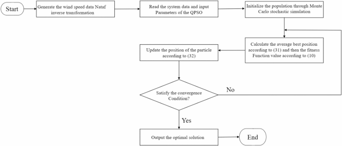
The flowchart of Quantum-behaved Particle Swarm Optimization.
Based on their exceptional qualities and prior achievements in related issues, the metaheuristic algorithms Grey Wolf Optimizer (GWO) and Quantum-behaved Particle Swarm Optimization (QPSO) were chosen to optimize the T-SFIS, GBM, and DT models. With just a few control settings, GWO is easy to implement and offers a good balance between exploration and exploitation. It was inspired by the hunting behavior of gray wolves. When it comes to forecasting the tensile strength of recycled concrete10 and solving routing issues50, this method has demonstrated excellent performance in optimizing predictive models in civil engineering. However, QPSO, a more sophisticated form of PSO, uses quantum mechanical concepts to provide faster convergence and better avoidance of local optima, making it appropriate for high-dimensional problems with intricate nonlinear relationships, like steel structure failure37 and concrete property prediction40. In contrast to more conventional techniques like grid search, these two algorithms were chosen for the current study due to their capacity to optimize the hyperparameters of machine learning models and enhance prediction accuracy.
Developing ensemble and hybrid models
Three distinct prediction models T-SFIS, GBM, and DT were integrated with metaheuristic optimization algorithms, GWO and QPSO, in three configurations to establish a novel methodology for evaluating the efficacy of the developed frameworks: i) individual mode (T-SFIS, GBM, DT), ii) hybrid mode (T-SFIS + QPSO = TSQP, GBM + QPSO = GBQP, DT + QPSO = DTQP, T-SFIS + GWO = TSGW, GBM + GWO = GBGW, DT + GWO = DTGW), and iii) ensemble mode (DT + GBM + T-SFIS = DGT). The primary objective of this research is to construct hybrid frameworks by integrating the principal prediction models of T-SFIS, GBMBoost, and DT with two optimization methods, hence introducing a novel methodology for tuning the estimation models. Optimizers endeavor to modify the programming procedures of models throughout the modeling phase. Some arbitrary parameters exist in the algorithms of models to which they are optimized. Consequently, by identifying the causal state variables of models at optimal levels, the models can operate at peak performance and accurately simulate the Strength features of HPC mixtures.
Conversely, ensemble methods are learning algorithms that integrate numerous distinct machine learning (ML) models to improve predictive performance45. The outcome is a conclusive model that surpasses the separate models. Ensemble approaches encompass bagging and boosting. Bagging seeks to enhance classification by amalgamating predictions from independently trained models within a randomly generated training set. The bagging method involves constructing multiple independent predictors and calculating the average of the estimators. It provides a predictor with reduced variance in comparison to independent predictors. Boosting is an ensemble meta-algorithm that amalgamates a collection of weak classifiers to construct a robust classifier. Incrementally construct the ensemble by continuously training new models and emphasizing misclassified training instances from prior models. The estimators are developed successively to minimize the bias of the final aggregated estimator. Figure 9 illustrates the schematic representation of the development of hybrid and ensemble models.

An overview of the hybrid and ensemble methodologies used to describe the Strength properties of HPC mixtures.
K-Fold cross-validation and sensitivity analysis
K-fold cross-validation is frequently employed to mitigate the random sampling bias linked to training and to maintain data samples. Kohavi’s evaluation indicates that the 10 × validation method offers dependable variance with low computational time46,47. The model’s performance in classifying the fixed dataset into 10 subsets is evaluated using a tenfold cross-validation technique. For testing reasons, he selects a certain portion of the data, while utilizing the remaining subset in each of the 10 rotations for model building and validation to train the chosen model. The test subset is analyzed to verify the algorithm’s accuracy. The algorithm’s accuracy is expressed as the mean accuracy derived from 10 models throughout 10 validation iterations. The sensitivity analysis of inputs is acknowledged to diminish the cost function throughout the modeling phase and mitigate biases that arise in computational stages. Consequently, the SHapley Additive exPlanations (SHAP) methodology48,49 was employed. Figure 10 illustrates the SHAP sensitivity analysis for the current research modeling work. According to plot (a) in Fig. 10, the superplasticizer and the water to binder ratio (W/B) are the primary factors influencing CS, significantly altering CS values more than other variables. In Fig. 10 plot (b), the parameters of the fine to total aggregates ratio (s/a), fly ash, and superplasticizer are among the most influential factors affecting the slump flow values in the slump test.

Sensitivity analysis for modeling (a) CS and (b) Slump.
Predictive performance evaluation indicators
To improve the predicted accuracy of the Gradient Boosting Machine (GBM) for HPC strength parameters, hybrid models GBQP and TSQP were created. Because of the intricacy of HPC mix design and the nonlinear interactions between inputs (such as silica fume and water-to-binder ratio), additional optimization is required beyond the grid search of regular GBM. By combining GBM with metaheuristic methods, such as Quantum-behaved QPSO for TSQP and GWO for GBQP, hybridization improves model fit to the 191 HPC dataset by optimizing hyperparameters. Hybridization is required since it can overcome GBM’s shortcomings in identifying complex patterns. GBQP attained R2 = 0.998, RMSE = 1.226 MPa for CS, and TSQP recorded R2 = 0.984, RMSE = 3.233 mm for slump flow, which represents 8–10% improvements above normal GBM (R2 = 0.92, RMSE = 3.45 MPa for CS; R2 = 0.90, RMSE = 5.67 mm for slump flow).
The subsequent indicators are employed to assess the efficacy of the pertinent models. The indicators comprised the mean absolute error (MAE), coefficient of determination (R2), root mean squared error (RMSE), variance account factor (VAF), and objective detection metric (OBJ), calculable by Eqs. (27)–(31):
$${R}^{2}={(\frac{{\sum }_{d=1}^{D}\left({n}_{d}-\overline{n }\right)\left({c}_{d}-\overline{c }\right)}{\sqrt{\left[{\sum }_{d=1}^{D}{\left({n}_{P}-n\right)}^{2}\right]\left[{\sum }_{d=1}^{D}{\left({c}_{d}-\overline{c }\right)}^{2}\right]}})}^{2}$$
(27)
$$RMSE=\sqrt{\frac{1}{D}{\sum }_{d=1}^{D}{\left({c}_{d}-{n}_{d}\right)}^{2}}$$
(28)
$$MAE=\frac{1}{D}\sum_{d=1}^{D}\left|{c}_{d}-{n}_{d}\right|$$
(29)
$$VAF=\left(1-\frac{var({n}_{d}-{c}_{d})}{var({n}_{d})}\right)\times 100$$
(30)
$$OBJ=\left(\frac{{n}_{train}-{n}_{test}}{{cn}_{train}+{n}_{test}}\right)\frac{{ MAE}_{test}+{RMSE}_{train}}{1+{R}_{train}^{2}}+\left(\frac{{2n}_{train}}{{n}_{test}+{n}_{train}}\right)\frac{{RMSE}_{test}-{MAE}_{test}}{1+{R}_{test}^{2}}$$
(31)
where \({n}_{d}\) determines the measured value, \(\overline{n }\) is the mean of the measured value, d shows the samples’ number, \({c}_{d}\) indicates the predicted value, \(\overline{c }\) determines the mean of the predicted values, and \(D\) is the data set’s number.
Because of its strong performance in regression tasks, especially when it comes to modeling nonlinearT1 complicated nonlinear interactions in the design of HPC mixes, the GBM was chosen as the foundational framework for the GBQP and TSQP models. GBM’s iterative boosting method, which adds weak learners one after the other to minimize a loss function, is ideal for capturing the complex relationships between Strength parameters (CS and slump flow) and HPC constituents (such as fly ash, silica fume, and water-to-binder ratio). Furthermore, GBM’s adaptability in hyperparameter tuning allows it to work with metaheuristic optimization methods such as Quantum-behaved QPSO and GWO, allowing for the creation of extremely accurate hybrid models (GBQP and TSQP). GBM is a perfect fit for this study since it provides a mix between interpretability and performance when compared to other sophisticated models like XGBoost and CatBoost.
For a relatively small dataset of 191 HPC mixtures, hybrid models integrating T-SFIS, GBM, and DT with GWO and QPSO were chosen because, even with limited data, they were able to capture complex nonlinear relationships between concrete components like water-to-binder ratio, silica fume, CS strength properties, and slump flow. Compared to conventional grid search techniques, metaheuristic algorithms like GWO and QPSO improve model performance by adjusting hyperparameters and lower the chance of overfitting through global search capabilities. This study’s use of tenfold cross-validation guarantees a thorough assessment and lessens biases brought on by limited sample sizes.
Metaparameter tuning process
Two metaheuristic algorithms, GWO and Quantum QPSO, are utilized in this study to tune the metaparameters of the suggested models (GBQP, TSQP, and DGT) in order to maximize their performance. In order to estimate CS and slump flow, the tuning method aimed to minimize prediction errors (measured by RMSE) and optimize model accuracy (measured by R2). Each model’s ranges were designed to balance exploration and exploitation during optimization, and the metaparameters were carefully chosen based on their influence on the model’s performance.
The number of trees (n_estimators: 50–200), maximum depth (max_depth: 3–10), and learning rate (learning_rate: 0.01–0.2) were among the tuned metaparameters for the GBQP model. We optimized the regularization parameter (C: 0.1–100), epsilon (epsilon: 0.01–1.0), and kernel parameter (gamma: 0.1–10) for the TSQP model. Together, the DGT model necessitated adjusting the weights of each learner (weights: 0.1–1.0) and the number of base learners (n_learners: 5–20). Whereas QPSO employed a swarm size of 50 particles and 100 replicates, the GWO algorithm was set up with a population size of 30 wolves and 100 replicates. As explained in Section “2.10”, both algorithms used tenfold cross-validation to iteratively adjust hyperparameters within predetermined ranges in order to minimize the RMSE on a validation subset (20% of the dataset). When compared to the default settings (i.e., scikit-learn default hyperparameters: n_estimators = 100, max_depth = 3, learning_rate = 0.1 for GBQP; gamma = 1.0, C = 1.0, epsilon = 0.1 for TSQP), the optimization procedure dramatically enhanced the model’s performance. The performance of the models with the default and optimized hyperparameters is compiled in Table 3, which also demonstrates how well GWO and QPSO work to improve prediction accuracy. For instance, the RMSE of the TSQP model for slump flow dropped from 5.891 mm to 3.233 mm, and the RMSE of the GBQP model for CS dropped from 2.547 MPa (default) to 1.226 MPa (optimized).


