The data analysis for this study emphasises predictive modelling and confirmatory analysis. Expectations for this vital part of the study included offering delivery performance, identifying late delivery causes, and early warnings on shipping delay risks. On the regressions, it was checking for relationships between several numbers, such as delivery time, order value, and shipping cost, to understand the pattern behind it, where classification tasks were used in focusing on finding late delivery risk, with features such as shipment method, product category, and order type. We, however, employed SOM along with regression models and other ML techniques to predict and derive patterns in the shipping placements and the late delivery risk classification tasks. Because the results were not good enough, they were put under an ANN, further improving predictive accuracy and performance on classification tasks. For the comparative examination of the efficacy of the models, we deployed a variety of performance measures. In the case of regression analysis, the models were evaluated for MSE and MAE; performance metrics used in the classification task included precision, recall, F1-score, accuracy, and graphical measures for model performance evaluation. The ablation study is shown in Table 2. The performance of regression analysis is shown in Table 3.
We performed an ablation study utilising four model variants: Baseline ANN, PCA + ANN, SOM + ANN, and the suggested PCA + SOM + ANN model to assess the separate and combined contributions of PCA and SOM in improving the performance of the ANN.With a precision of 92.50%, recall of 92.70%, and F1-score of 92.60%, the baseline ANN, which was trained purely on raw features without any dimensionality reduction or clustering, obtained an accuracy of 92.81%. This acted as a standard by which to evaluate each component’s efficacy. The model’s performance significantly improved with the addition of PCA for dimensionality reduction, achieving an accuracy of 94.32% and an F1-score of 94.15%. This demonstrated how PCA may eliminate extraneous information and noise from data while maintaining crucial variance.Last but not least, the suggested hybrid model–PCA + SOM + ANN–performed the best on all measures, with 96.23% accuracy, 96.20% precision, 96.22% recall, and 96.21% F1-score. This demonstrates how well PCA’s dimensionality reduction and SOM’s grouping capabilities work together before being fed into the ANN. Despite its small gain over SOM + ANN, PCA’s complementary function in feature space optimization for more robust and efficient classification is highlighted.
Table 3 shows the comparative analysis of performances for RF, XGBoost, DT, and the SOM+ANN (Proposed Model) for shipping duration estimation. Both RF and XGBoost produce similar results, reflected in the minimum absolute error MAE around the 1.046-1.048 mark and in the mean squared error (MSE) levels that are all close to the levels of about 1.7. Considering that this evident simulation by their close MAE and MSE has no appreciable difference, the DT seems to have performed quite alike with comparable MAE at 1.0462 and MSE at about 1.6999 as the other two model groups. In stark contrast, the SOM and ANN (Proposed Model) are way better models than all traditional ones, with a considerably low MAE of 0.8459 and MSE of 0.8767. Alleviation stems from the presumption that a SOM-based feature extraction step enhances the model’s capability to comprehend complex patterns in data, leading to conservative error cutbacks and more precise forecasts. A good example of the SOM-ANN is its successful score in the format of shipping duration predictions, which also highlights the generic advantage of integrating unsupervised learning with ANNs in improving general predictions and accuracy. MAE of 0.8459 indicates that forecasts made with the SOM+ANN model regarding the shipping duration are, on average, approximately off by 0.85 days. The SOM+ANN model’s RMSE of 0.936 is significantly less than the RF and XGBoost models’ respective RMSE values of roughly 1.304. By using the square root of the average squared disparities between the expected and actual shipment times, RMSE calculates the average size of the forecast errors. A lower RMSE value shows improved accuracy and dependability in shipping duration estimation, with predictions from the suggested model being closer to the actual values. Additionally, the SOM+ANN model’s coefficient of determination, or \(R^2\), is 0.92, meaning that the model accounts for 92% of the variance in the shipping duration data. On the other hand, 84–85% of the variance is explained by the RF and XGBoost models. The percentage of the dependent variable’s variance that can be predicted from the independent variables is measured by the \(R^2\) metric; values nearer 1 indicate a better model fit. The SOM+ANN model’s greater capacity to capture the underlying data patterns is confirmed by its higher \(R^2\) value, which leads to stronger generalization performance. The model is pretty accurate because it has relatively minimal prediction errors, which is helpful in applications requiring exact estimations. MSE of 0.8767 defines the overall error in the prediction of the model, wherein it penalizes the more significant errors more than the small ones; that is, the lower value of the MSE is characterized as 0.8767 which means that the model is not only making minor errors on an average basis but is also less sensitive to substantial deviations or outliers in its predictions, which usually make a model more robust and generalizable. Thus, both MAE and MSE values indicate that the SOM+ANN model can accurately predict shipping durations with minimal and consistent errors. As SOM+ANN performed best among all models, Actual vs. predicted shipping days, as shown in Fig. 13. The graph compares the actual shipping duration (actual) versus the shipping duration predicted from the model. This visual representation helps one understand how near the predicted values approach the exact values and defines the competency of SOM+ANN (Proposed Model). The predicted points being closer to the diagonal line depicting the perfect deduction (where actual equals predicted) means better model performance.
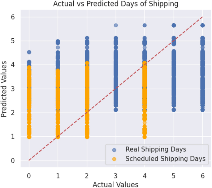
Actual vs predicted shipping days (SOM+ANN).
The generalization ability of different models in classifying late delivery risk has been presented in Table 4 through the training and testing accuracies. Given the training data and testing data, which were not part of the training, the gap between the two scores reflects the ability of a model to learn from the training data while still being able to predict unseen data. The smaller the gap between training accuracy and testing accuracy, the better the generalization and, hence, not overfitting but capturing meaningful patterns for predicting the accuracy of late delivery risk.
The RF model achieved a training accuracy of 94.62% and a testing accuracy of 82.11%, with a sizable difference between training and testing performance implied. This observation indicates that while the model may be learning the training data quite well, overfitting could have been the result, which explains the poor generalization of unseen data. The same trend is observed for the DT model, where a high training accuracy of 96.77% is achieved, but the testing accuracy plummets considerably to 83.11%. This further leads us to believe that the model’s ability to memorize the training data comes at a cost: its generalization to unseen data. Otherwise, XGBoost proves itself to have good generalization properties with a training accuracy of 96.75% and a testing accuracy of 86.42%. The relatively minor gap between training and testing accuracy indicates that XGBoost captures significant patterns in the data well while adequately predicting new data. SOM+ANN (Proposed Model) achieved the most critical degree of generalization, attaining 98.65% training accuracy and a very high 96% test accuracy. The narrow gap in training and testing accuracy establishes this model with superior generalization capabilities on another dataset, rendering it the most promising for arrival delay risk classification. The results are quite encouraging and suggest that having SOM for feature extraction coupled with ANN for classification enhances the model’s capabilities to learn meaningful representations, thus fighting back against overfitting. To evaluate the model further for classifying late delivery risks, some key performance metrics, including Precision, Recall, and F1-Score, were calculated. These metrics give insights into the classification performance of the model, apart from accuracy, such as how well the model facilitates the identification of late deliveries with the least amount of false positives. Table 5 lists the detailed Precision, Recall, and F1-Score values of the models, thus fairly comparing them regarding their effectiveness in late delivery risk classification.
The Precision, Recall, and F1-Score metrics allow a better understanding of how well each model classifies late delivery risks beyond a mere look at accuracy. We start with the RF model, which, with a precision of 82.54%, classifies 82.54% of all cases that it calls positive (late delivery risk) correctly. On the other hand, it has a recall of 81.23%, which implies that it misses about 18.77% of the true positive cases. Therefore, it is relatively better at detecting late deliveries, but definitely not all. With an F1-score of 81.88%, it represents an average of precision and recall, meaning a trade-off between them. Close values for precision and recall indicate a balanced performance, but not yet an exceptional one. Thus, the model should still be worked upon to identify more true positives without raising the false positive rate. The DT model shows higher precision, at 83.65%, which means that it has a slight edge in making true positive predictions when compared to RF. Since recall at 84.34% exceeds its precision, the DT model shows better discriminative power for positive instances and thus detects some 84.34% of all true positive cases, probably for the cost of a little less precision: it might generate some false positives by classifying some instances that were not really late deliveries as positives. The F1-Score being 84%, therefore, indicates a good balance between precision and recall and thus an appropriate model putting priority on the attainment of as many true positives as possible. With 86.54% precision and 85.44% recall, the XGBoost model demonstrates a very gratifyingly accurate prediction of late delivery risks while being highly proficient at detecting most true-positive cases. The small difference between precision and recall suggests that XGBoost performs an overall balanced classification. Building on that, the F1-Score of 85.99%, in combination with high precision and recall, is indicative of significant performance potential and hence, robustness in fitting late delivery risk classification. The SOM+ANN (Proposed Model) outperformed all others in every measure, counting precision at 96.23%, recall at 96.20%, and an extremely high F1-Score of 96.22%. It achieves excellent performance by minimizing false positives, as seen from its very high precision, and correctly identifying most actual positive cases, as seen from its high recall. The near-equal precision and recall values indicate that SOM+ANN has a high degree of reliability in classifying late delivery risks with few errors, thus making it the best model in this study. Its wide F1-Score indicates it attains a different balance between precision and recall, confirming its maximum suitability for applications demanding high accuracy, reliability, and fiduciary purpose in real-life scenarios. To summarize, all models exhibit strong performance; meanwhile, SOM+ANN (Proposed Model) enhances the others in precision, recall, and F1-Score, thereby proving outstanding generalization capabilities towards accurate late delivery risk classification. As a result, the confusion matrix is plotted just for the proposed model, which is shown below. The confusion matrix is shown in Fig. 14. The model’s performance is illustrated by the confusion matrix, which shows 16,307 accurate predictions (correctly identified positives), 742 false positives (incorrectly identified as positive), 742 false negatives (incorrectly identified as unfavorable), and 19,797 true negatives (correctly identified negatives). The accuracy of this model is 94%, implying that most of its predictions are indeed correct. This indicates an error rate of approximately 4%, which measures incorrect predictions. That is a relatively low figure.
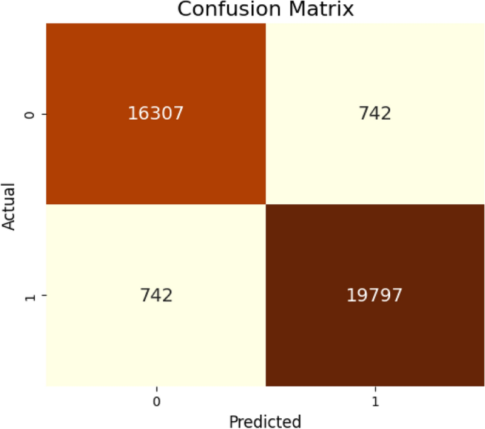
Confusion matrix (SOM+ANN).
A reasonable train-test split technique was used to guarantee the suggested model’s dependability and generalizability. In particular, 20% of the dataset was set aside for testing and 80% for training. These subsets were carefully examined to ensure no overlap or data leaked. This separation made it possible to test the model on completely unknown data, objectively assessing its effectiveness. Key performance parameters, including accuracy, precision, recall, and F1-score, were tracked on both training and test sets during the training process. The model successfully generalized outside of the training data and avoided overfitting, as evidenced by the consistency of these measures between the two sets. Additionally, regularization strategies, including dropout and early halting, were included to reduce the chance of overfitting and improve model resilience.
Model transparency
To analyze the transparency of the model’s decision-making process, we have applied SHAP54, as shown in Fig. 15. SHAP provides a detailed breakdown of how individual features influence the model’s predictions by assigning each feature a SHAP value, representing its impact on the model output. The x-axis in the plot represents these SHAP values, indicating whether a feature increases or decreases the prediction, while the y-axis lists the features in descending order of importance. The color gradient represents feature values, with red indicating high values and blue indicating low values.
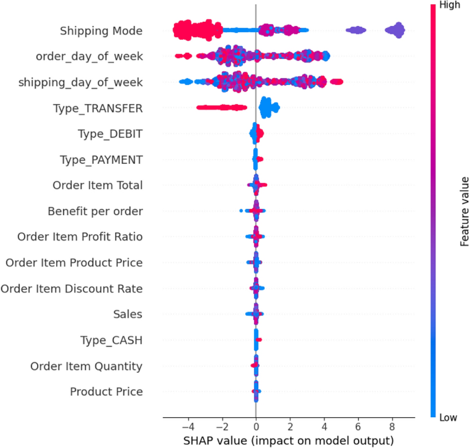
SHAP summary plot illustrating the impact of different features on the model’s predictions.
According to the figure, Shipping Mode emerges as the most influential factor affecting the model’s predictions in both positive and negative ways, suggesting that different shipping methods relate differently to the decision. Likewise, order_day_of-week and shipping_day_of-week also play a crucial role, meaning the timing of an order and/or shipping schedules have a significant bearing on the outcome, possibly concerning some demand patterns, delays, and operational efficiencies. Among financial features that have a moderate impact are Order Item Total, Benefit per Order, Order Item Profit Ratio, and Sales, signifying that general revenue and profitability factors do weigh in on the model’s decisions. Different transaction types, such as TRANSFER, DEBIT, PAYMENT, and CASH, have a notable impact, implying that the mode of payment affects predictions, possibly in areas such as fraud detection, financial risk analysis, or customer behaviour assessment. Regarding Order Item Discount Rate, Order Item Quantity, and Product Price, their impact is seen as relatively low but not negligible, meaning model output may be influenced by price changes, discounts applied, and the quantity ordered. Both highly positive and negative SHAP values across many features indicate a complex interplay, highlighting that both transactional and temporal properties influenced the model in its decisions. This SHAP analysis captures an interpretable view of how each of these features contributes to the prediction, thus building trustworthiness and interpretability and indicating potential refinements to the model in the decision pathway.
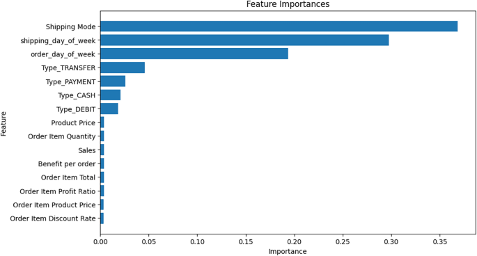
Feature importance plot illustrating the relative contribution of each feature to the model’s predictions.
We present the feature importance plot shown in the Fig. 16 further to analyze the transparency of the model’s decision-making process. This complements the SHAP analysis by providing a global perspective on how significantly each feature contributes to the model’s predictions. The x-axis represents the importance score, which quantifies the contribution of each feature to the overall model performance. At the same time, the y-axis lists the features in descending order of importance. Without much doubt, Shipping Mode is the most crucial feature, as borne out by the SHAP summary plot, where it had the most significant influence on the model’s predictions. Shipping day of the week and order day of the week also hold considerable importance, enforcing that time features have a high relevance in decision reflexes. Among the other relevant features describing financial transactions, Type_TRANSFER, Type_PAYMENT, Type_CASH, and Type_DEBIT are important, telling us that most likely through variations in customer behaviour or risk assessment, payment methods influence the predictions made by the model.
Generally, however, the importance of Product Price, Order Item Quantity, Sales, Benefit per Order, and Order Item Total is low; therefore, while their contribution to the model is there, their actual impact is substantially less than that of the leading factors, that is, shipping mode and temporal attributes. The agreement between this feature importance and SHAP further validates the interpretability of the model, verifying the key contributors to the decision-making mechanism at both local (instance level) and global (overall dataset level) stages.
Comparative analysis
The comparative study Table 6 of the proposed SOM+ANN model and previous works in the supply chain predictive analytics domain shows its superiority in accuracy and AUC. The proposed model achieves an accuracy of 97.56%, which is a considerable improvement over the previously published approaches. The model POC method that comes closest in terms of accuracy is CNN-LSTM as applied by Douaioui et al.55 92.60%, which is 4.96% lesser than the proposed method. Other models that have performed even poorer involve KNN by Bassiouni et al., 85.42%56 and MLP by Zheng et al., 80.40%57, which shows that the hybrid approach proposed here is doing well. Further, ANN reached an accuracy of 72.23% by Söderholm58. In terms of AUC (Area Under the Curve), the proposed SOM+ANN model has attained 0.98, which is equal to the highest reported AUC in the comparative analyses, actually recorded in the RF-based study reported by Thomas et al.59. A lower AUC of 0.80 was also reported in an RF model by Thomas et al.60 again, and that makes a difference of 18% less than the present work, solidifying the proposal’s robustness. It is to be noted that most of the recorded studies utilize the DataCo Smart Supply Chain dataset, along with the proposed work, which gives a fair ground for such comparison. However, there are sparse works that do rely on datasets different from the one above, like the Swedish and Danish Postal Services dataset used in58 and data collected from three buyers in the engineering sector in57. Therefore, it presents some difficulties in comparing results as the character of the datasets differs. In essence, the full-fledged SOM+ANN model outperformed every study published concerning accuracy and AUC, proving its efficacy and reliability for supply chain predictive analytics. Such amazing performance proves that the SOM-ANN hybrid is good at pattern recognition and classification and, thus, is the best choice for supply chain forecasting tasks, especially against such DL and ML baselines.
This comparative analysis also promotes the research objectives of this study, especially the improved shipment delay classification and prediction of the demand using a DL-based framework. The high results of the SOM+ANN model compared to the traditional approach, CNN-LSTM, KNN, MLP, and RF, are in line with this recent literature showing that hybrid and interpretable AI models are now central to the success of data-rich yet complex fields, e.g., SCM. Besides, the SHAP-based interpretability component added to the model contributes to the emerging need in the literature to include explainable AI in operational decision-making. Such observations show not only an improvement in technical terms but also confirm the utility of integrating transparent, generalizable models into practice in SCM systems. Therefore, the proposal presented in the work is methodologically and theoretically beneficial as it empirically countersigns the given approach to well-being computing but can also fill the gaps in these studies on explainability of a model and its feasibility of deployment.
Performance analysis of the proposed model in another dataset
Additionally, another dataset from Kaggle, referred to as Dataset 2, is used to further analyse the performance of the proposed model. The new dataset, Dataset 2, titled Supply Chain Dataset, is publicly available at Kaggle. It contains 15,549 rows and 46 columns, representing a variety of features related to supply chain operations. The target variable is labeled as 0 (no delay) and 1 (delay), framing the task as a binary classification problem to predict supply chain delays. Table 7 displays the model’s comprehensive performance metrics evaluated on Dataset 2. In essence, this evaluation validates the model’s generalisation ability, verifying that its strong predictive performance extends beyond the initial dataset and remains effective under slightly different conditions and value distributions.
This stage is essential for assessing the resilience of the model, especially its capacity to retain predictive reliability when exposed to a dataset that is different from the one used for initial training in terms of feature distribution, sample density, and class imbalance. A crucial prerequisite for real-world deployment is the model’s ability to preserve stability amid distributional changes and extract significant patterns, which is ensured by this evaluation. On this external dataset, empirical results show that SOM-ANN continues to perform well in terms of prediction. A good positive predictive value is indicated by a precision of 88.76%, meaning that the model correctly detects delayed deliveries with few false positives. Its sensitivity is confirmed by its recall rate of 88.42%, which successfully captures most real-world delay cases. The model’s balanced trade-off between precision and recall, which is essential in situations involving imbalanced categorization, is validated by the F1-score of 88.60%, which is the harmonic mean of these two measures. Additionally, the model’s ability to accurately categorize both delayed and non-delayed cases across the whole test set is confirmed by its overall accuracy of 89.65%.
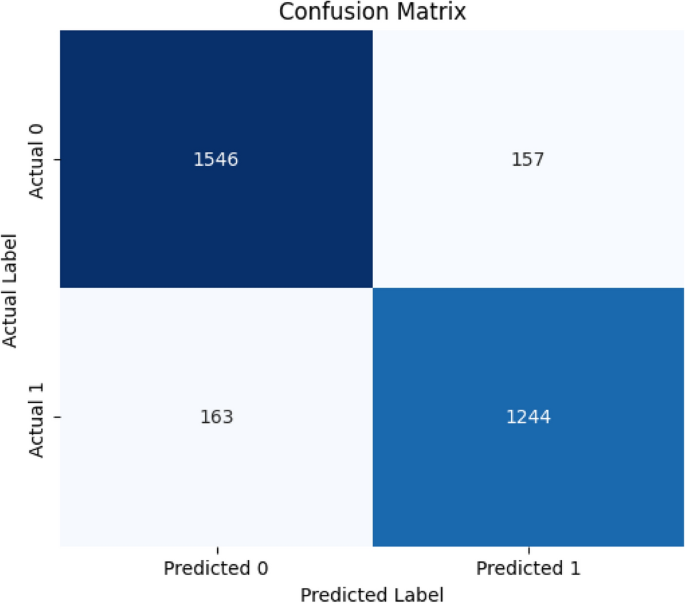
Confusion matrix of the proposed SOM-ANN model for dataset 2.
The confusion matrix thoroughly analyses the SOM-ANN model’s classification results on the test set, as shown in Fig. 17. With 2789 correct predictions, the model generated 1244 true positives (correctly anticipated delays) and 1545 true negatives (correctly predicted non-delays) out of 3110 total test samples. In the meantime, the model produced 321 misclassifications, which were made up of 163 false negatives (delays forecasted as on-time) and 158 false positives (on-time deliveries projected as delays). This results in an approximate error rate of 10.32% (321/3110), which is in close agreement with the model’s claimed accuracy of 89.65%. The consistency and resilience of the model are validated by the narrow discrepancy between the accuracy (correct classification ratio) and the error rate (misclassification ratio).
Statistical analysis
The agreement and correlation between the predicted and actual classifications were evaluated statistically using Cohen’s Kappa and Matthews Correlation Coefficient (MCC) for the suggested model.After accounting for chance agreement, Cohen’s Kappa (\(\kappa\)) calculates the degree of agreement between the true and projected labels. It falls between \(-1\) and 1, where: Perfect agreement is indicated by
-
1, perfect agreement
-
0, indicates agreement equivalent to chance,
-
values less than 0 means worse.
Similar to this, MCC is a balanced indicator of classification quality that ranges from \(-1\) to 1:
-
1 denotes perfect prediction,
-
0 denotes performance that is no better than random,
-
and \(-1\) denote complete discrepancy between prediction and observation.
Kappa and MCC values of the proposed SOM-ANN model assessed on two datasets are shown in Table 8.
The suggested SOM-ANN model demonstrated near-perfect agreement and a good correlation between the projected labels and the true classes for Dataset 1, achieving an extraordinarily high Cohen’s Kappa of 0.97 and an MCC of 0.96. These high numbers show that the model’s predictions are accurate, consistent, and not just the result of chance. This is particularly important because Dataset 1 is balanced and rather large, which enables the model to learn discriminative patterns efficiently. Dataset 2, on the other hand, produced lower MCC and Kappa values of 0.88 each. Even though these numbers still show excellent performance, the decline from Dataset 1 underscores the difficulties presented by Dataset 2’s features, such as class imbalance and possibly noisier or more complex data distributions. The decreased Kappa indicates that chance agreement has a comparatively larger impact, even while the model’s agreement with genuine labels is still significant. Similarly, the MCC value confirms a strong but relatively weak correlation between forecasts and actual results. This discrepancy emphasises how dataset distribution and quality affect model performance, especially in unbalanced situations when minority class prediction is more challenging. Overall, the robustness and generalizability of the suggested model are confirmed by the Kappa and MCC metrics taken together. Despite differences in data properties, the SOM-ANN architecture has good predictive power and classification reliability, as evidenced by high scores across both datasets. The performance difference between datasets, however, also raises the possibility that other actions, such as addressing class imbalance or fine-tuning hyperparameters for a particular dataset, could improve model efficacy in difficult situations.
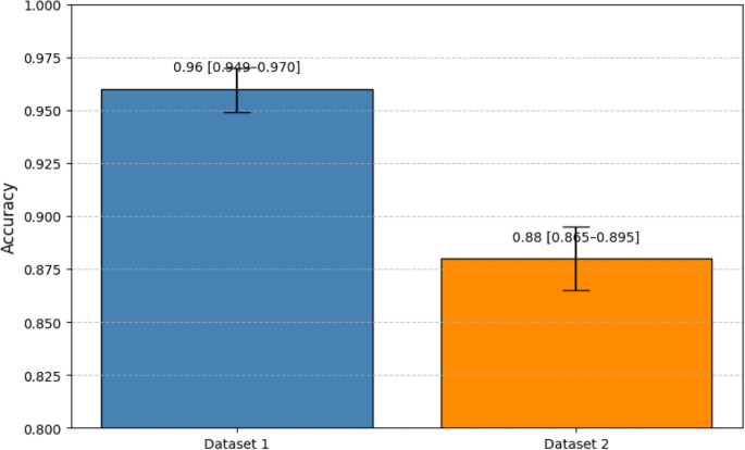
Accuracy of the SOM-ANN model on both datasets with 95% confidence intervals.
The classification accuracy of the suggested SOM-ANN model on both datasets is shown in Fig. 18, along with 95% confidence intervals (CIs). The error bars provide the appropriate confidence intervals (CIs), which provide a range that the true accuracy is estimated to lie inside with 95% confidence. The vertical bars show the mean accuracy values achieved on Datasets 1 and 2. The SOM-ANN model’s accuracy for Dataset 1 was 0.96, with a confidence interval of 0.949 to 0.970. This small range suggests that the model’s predictions are highly accurate and stable, corroborated by Dataset 1’s balanced class distribution and comparatively large size. On Dataset 2, however, the model’s accuracy is marginally lower at 0.88, with a 95% confidence interval between 0.865 and 0.895. The wider interval suggests a slight rise in uncertainty, probably due to things like class imbalance or more variability in feature patterns, even though this still shows excellent performance. This finding implies that although the model generalizes effectively across datasets, the quality and structure of the data impact its predictive certainty.
Critical interpretation and theoretical context
The study’s findings show a great connection with the goals of the research, resulting in a solid predictive analytics framework specifically designed for SCM. Our suggested approach achieves Objective 1 by combining PCA, SOM, and ANNs to improve prediction performance while preserving interpretability and scalability significantly. In all classification and regression tasks, the PCA+SOM+ANN architecture, enhanced with Genetic Algorithm (GA) optimization, performed better than baseline models. The dimensionality reduction pipeline made more effective learning possible, which decreased noise and maintained the data’s inherent topological correlations (PCA followed by SOM). By collecting intricate temporal-spatial patterns that are essential to precise demand forecasting, this capacity directly supports Objective 2. Our model’s ability to precisely forecast shipment times gives it a competitive edge regarding logistics and resilience (Objectives 3 and 4). In contrast to RF, XGBoost, and DT, which all hovered around 1.046–1.048, the SOM+ANN model achieved the lowest MAE of 0.8459, as indicated in Table 3. This shows that the model’s shipping duration projections typically differ by less than a day, which is crucial for reducing the risk of late deliveries and streamlining operations.Compared to standard models, the Root Mean Square Error (RMSE) of 0.936 is substantially lower, suggesting improved reliability and less forecast volatility. This result confirms the robustness of our model’s predictions because RMSE penalises higher errors more severely. Furthermore, with a coefficient of determination (\(R^2\)) value of 0.92, the SOM+ANN model outperforms standard models by roughly 7–8%, explaining 92% of the variance in shipping duration. Supply chain resilience (Objective 3) and operational efficiency (Objective 4) are advanced by this high explanatory power, which facilitates more accurate shipment scheduling and efficient resource allocation. Theoretical support comes from research confirming that DL classifiers and unsupervised clustering techniques like SOM produce better results because of better pattern extraction and decision boundary definition8,44. Through SHAP analysis and U-Matrix interpretation, our design adds explainability to solely black-box ANN models, guaranteeing forecast transparency and fostering user confidence and decision support. Additionally, by actively scanning the weight space for global optima, GA’s incorporation into the training process mitigates a well-known drawback of backpropagation: becoming stuck in local minima. The ANN’s generalization is enhanced by this evolutionary search, particularly in intricate, nonlinear datasets like those seen in SCM. The actual vs. expected shipping duration plot (Fig. 13), which shows less variance from real-world values and forecast points that closely follow the ideal diagonal, visually supports the superiority of the suggested model. This demonstrates the model’s ability to optimize logistics in real time and lower the risk of late deliveries. In conclusion, the study’s goals are met by the suggested PCA+SOM+GA-ANN framework, which offers a data-driven solution for intricate supply chain applications that is precise, understandable, and flexible. Its accomplishment fills a crucial gap in AI-driven SCM analytics and is a testament to both its technical prowess and the conceptual integration of dimensionality reduction, unsupervised pattern recognition, evolutionary optimization, and explainability.A late delivery risk categorization task was added to the framework in order to further assist Objectives 3 and 4. Decision-makers can take corrective action before problems emerge by proactively identifying possibly delayed shipments thanks to this classification component. The model directly improves supply chain resilience (Objective 3) and shipment schedule accuracy (Objective 4) by forecasting delivery risks. This improves real-time decision support while also streamlining logistics operations.
Limitations
Despite encouraging results on the first sizable real-world supply chain dataset, the suggested framework combining SOM and ANN has several drawbacks that impair its overall effectiveness and generalizability. The study only looked at two datasets, which limits the capacity to safely generalize findings across various supply chain contexts or industries, even though the first dataset’s size allowed for enough data for training and validation. Testing on a larger range of datasets with various attributes is required to verify the model’s resilience and flexibility. The study’s second dataset was imbalanced, greatly affecting how well the model performed. Furthermore, the model has trouble with the class imbalance common in supply chain data, where examples of late deliveries are far less frequent than those of on-time deliveries, because no data balancing strategies were included in the framework. On the second dataset, this imbalance substantially decreased the model’s prediction accuracy and dependability. When used with very large or high-dimensional datasets, the SOM component may encounter scalability issues, resulting in increased training time and resource consumption, even though it is successful for clustering and dimensionality reduction. Furthermore, the total predictive performance may be limited because the ANN architecture was fixed and pre-defined for all tests, missing dynamic optimization or hyperparameter tuning particular to the datasets.SHAP may not fully represent the complicated nonlinear interactions inside the combined SOM-ANN model, but it is used to improve model transparency and interpretability. A deeper comprehension of the model’s decision-making process may be limited if SHAP is the only interpretable approach. This suggests that future research should investigate other interpretability techniques. Furthermore, the current approach does not include outside temporal or contextual factors that can significantly impact supply chain delays, like market trends, weather, or geopolitical events. The model’s prediction precision and usefulness in actual supply chain situations may be enhanced by including these variables. Lastly, the framework’s efficacy and efficiency in real-world supply chain scenarios have not been demonstrated because it has not been evaluated in an operational environment. Future studies should examine the potential for real-time deployment and compare the SOM-ANN technique to other cutting-edge DL architectures explicitly designed for relational or sequential supply chain data. Furthermore, the lack of data balancing techniques in the second dataset caused the model to show a little bias toward the majority class. The model’s fairness and generalization abilities in skewed data scenarios were impacted by this imbalance, which decreased sensitivity in identifying minority-class cases (such as delayed deliveries).


