Our investigation aimed to assess the efficiency and robustness of the transfer learning approach using visual dynamic features to defend against ransomware attacks with limited datasets. This section consists of three components: experimental setup, evaluation metrics, and experimental results and discussion.
Experimental setup
The experimental setup of this study incorporates sophisticated tools and techniques to analyze ransomware using dynamic analysis techniques. The analysis environment used a cuckoo sandbox46 to execute and monitor diverse ransomware behaviors securely. The evaluation environment leveraged Google Colab Pro62 with 51 GB of RAM, offering robust cloud computing to manage resource-intensive experiments and model training. Python version 3.10.12 was used to take advantage of the latest features, with essential libraries such as TensorFlow63 and Keras64 to implement and train deep learning models, as well as Pandas65 and NumPy66 for data management and numerical computations. Preprocessing involves scripting workflows in Python and using Bash commands to analyze the input/output operations of the JSON reports and store the resulting data in a CSV file. Additionally, color-mapping techniques were employed on structured CSV data via a Python script to visually represent the behavioral patterns of ransomware and benign applications.
Dataset splitting and evaluation strategy
The final dataset comprises 1,000 image samples derived from structured behavioral features, with an equal distribution of 500 ransomware and 500 benign samples. To ensure robust evaluation, we applied an 80/20 stratified split, resulting in 800 samples used for training and 200 for validation. The validation set was used to monitor the performance of the model during training, guide early stopping, support learning rate adjustment, and not for final testing. Although no separate test set was used owing to the small dataset size, we ensured performance generalization by-
-
Stratified random sample splitting was used to preserve the class balance (50% ransomware and 50% benign) in both subsets.
-
Applying early stopping and ReduceLROnPlateau callbacks based on validation metrics to avoid overfitting.
-
Multiple runs were performed, and the results were compared across different models and data configurations (color vs. grayscale) for consistency.
This setup allowed us to optimize training while mitigating overfitting risks, ensuring that the results reflected the true model performance under controlled conditions.
To support the misclassification and interpretability analysis, we conducted additional evaluations of the trained model using the 200-sample validation set. These evaluations were used to generate confusion matrices and assess the generalization capabilities of the modelwhile maintaining controlled training-validation separation.
Evaluation metrics
To analyze and evaluate the results, we employed the precision, recall, F1 score, area under the curve (AUC), accuracy, and loss curve as performance metrics to assess the models for ransomware classification. However, accuracy was considered as the primary metric. The following equations (Eqs. (1)– (4)) describe the mathematical formulas for these metrics:
Before proceeding with the equations, we define the acronyms of the confusion matrices used in the formulas:
-
TP: True positive (correctly identified ransomware samples).
-
TN: true negative (correctly identified benign samples).
-
FP: False positive (benign samples incorrectly labelled as ransomware).
-
FN: False negative (ransomware samples incorrectly labelled benign).
Accuracy: Accuracy is a metric that calculates the ratio of correct predictions (including both true positives and true negatives) to the total number of observations in a dataset.
$$Accuracy = \frac{{TP + TN}}{{TP + TN + FP + FN}}$$
(1)
Precision: This measures the proportion of correctly predicted positive observations to the total number of predicted positive observations.
$$\Pr ecision = \frac{{TP}}{{TP + FP}}$$
(2)
Recall: This is also termed the sensitivity or true-positive rate, which measures the percentage of positive instances accurately classified and is calculated using the following formula:
$$\text{Recall} = \frac{{TP}}{{TP + FN}}$$
(3)
F1 score: F1 score combines precision and recall into a single metric, offering a balanced evaluation of false positives and false negatives.
$$F1 – measure = 2 \times \frac{{\Pr ecision~ \times \text{Re} call}}{{\Pr ecision + \text{Re} call}}$$
(4)
Area under the curve (AUC): The AUC metric evaluates the performance of a binary classifier by plotting a receiver operating characteristic (ROC) curve that shows a trade-off between true positives and false negatives at different thresholds. High AUC values indicate effective classification with minimal error.
Loss: Loss measures the error between the predicted and actual labels during training, with lower values indicating better model performance.
Results analysis
We performed a series of experiments based on the following: (1) experiments with pretrained models and (2) experiments with nontrained models. (3) Performance comparison between grayscale and color image datasets. (4) Comparison of robustness and computational efficiency (5) Model interpretability and visual analysis (6) Misclassification analysis and (7) Comparison with relevant existing studies.
Experiment with pretrained models based on color and gray image datasets
We trained six pretrained models with varying configurations, as listed in Table 4. The performance metrics (accuracy, precision, recall, F1-score, AUC, and loss) for the ransomware classification results are summarized in Tables 5 and 6 for both color and grayscale samples. The primary evaluation metric was accuracy, which was tracked across all the experiments to measure the effectiveness of each model.
ResNet50 emerged as the top-performing model, achieving 99.96% accuracy on the color dataset and 99.91% on the grayscale dataset. This 99.96% represents the highest training accuracy observed during repeated experiments (epoch 24). To further illustrate model behavior, a confusion matrix was generated from the validation set comprising 200 samples corresponding to the same training run. While training accuracy highlights the model’s optimal learning performance, the confusion matrix provides practical insight into its generalization and classification behavior on held-out data used during early stopping, not final testing. The consistently high precision, recall, F1-score, and AUC confirm ResNet50’s superiority.
EfficientNetB0 followed closely with an accuracy of 99.91% on the color dataset and 99.70% on the grayscale dataset, thereby showing strong generalizability. Xception and InceptionV3 also demonstrate high effectiveness but with slightly lower scores, indicating their robustness in handling ransomware detection tasks. Conversely, VGG16 and VGG19 exhibited relatively low performance metrics, particularly when transitioning from the color to grayscale datasets.
Based on the results from both datasets the color dataset consistently outperformed grayscale, with all models achieving higher accuracy on color samples. Consequently, color images were prioritized for subsequent analysis. Figures 3 and 4 further underscore ResNet50’s superiority, showing its high accuracy trajectory and the lowest loss trend compared to other models. This advantage is attributed to its deeper architecture and advanced feature extraction capabilities, enabling it to capture complex behavioral patterns effectively. In contrast, the shallower VGG models exhibited limitations in handling feature-rich ransomware data.
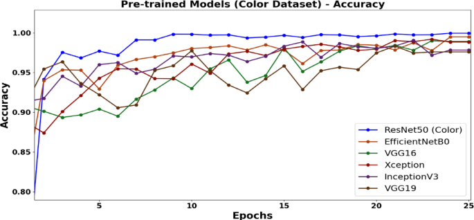
Accuracy trends for various pretrained learning models. The ResNet50 model demonstrates superior accuracy as the number of epochs increases.
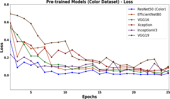
The loss trends of pretrained models show that reveals that the ResNet50 model consistently demonstrates the lowest loss as the number of epochs increases.
Experiment with non-pretrained models based on color and gray image datasets
The performance of the non-pretrained models was evaluated on both color and gray image datasets, as shown in Tables 7 and 8. The results revealed that the integrated CNN-GRU consistently outperformed other non-pretrained models across both datasets. For color images, CNN-GRU achieved the highest accuracy of 97.49% with a corresponding loss of 0.0579. Similarly, for gray images, an accuracy of 97.07% was achieved, with a loss of 0.0680. CNN-LSTM closely followed, demonstrating a slightly lower accuracy (96.94% for color and 96.80% for gray images) and greater loss than CNN-GRU. The standalone CNN model exhibited a performance similar to that of CNN-LSTM, achieving accuracies of 96.84% for color and 96.71% for gray images but with marginally higher loss values (0.0998 and 0.1045, respectively). The ANN consistently underperformed, showing the lowest accuracy (90.48% for color and 89.24% for gray images) and the highest loss values (0.2707 for color and 0.2853 for gray images).
The associated graphs in Fig. 5 further clarify the analysis of the performance of these models across various image types. The graph comprises two plots that evaluate the performance of various non-pretrained models over 15 epochs in terms of accuracy and loss. ResNet50 was included as a reference pretrained model, and it displayed superior and stable performance across all epochs, quickly converging to near-perfect accuracy and minimal loss. This demonstrates the advantages of transfer learning. Among the non-pretrained models, the CNN-GRU achieved the highest accuracy and lowest final loss, highlighting its strength in capturing spatial and sequential features. These results highlight the superiority of the pretrained and hybrid models for image-based ransomware classification.
The ANN demonstrated a limited learning capacity with lower accuracy and inconsistent loss trends. ANNs lack the ability to capture spatial and temporal dependencies, which likely accounts for their poor performances. CNN-LSTM demonstrated a similar structure to CNN-GRU but with less favorable results, possibly because of the relatively heavier computational burden of LSTM for this task.
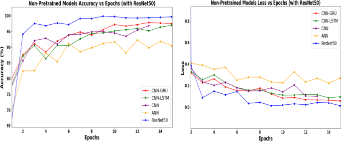
Comparative performance of non-pretrained models and ResNet50 over 15 epochs.
Performance comparison between color and grayscale datasets
The comparative results in Table 9; Fig. 6 reveal that all the models (pretrained and nontrained) performed slightly better on the color datasets than on the grayscale datasets in terms of accuracy and loss drop.
However, the performance differences were negligible for most models.
-
ResNet50 achieved the highest accuracy for both datasets, with only a minor difference of 0.05%, and maintained the lowest loss gap (0.0033%), demonstrating its superior performance across both datasets and among all the models. EfficientNetB0 also demonstrated strong results, with a slight decrease in accuracy (0.12%) and a modest increase in loss (0.0114) for gray images.
-
Among the non-pretrained models, the CNN-GRU outperforms the CNN-LSTM and CNN, with a relatively small accuracy gap (0.42%) and minimal loss difference (0.0101), whereas the ANN showed the largest performance decline, with a 1.24% decrease in accuracy and a 0.0146 increase in loss for gray images.
-
Notably, CNN-LSTM is the only model with a marginally lower loss for gray images, indicating its unique adaptability to grayscale inputs.
-
Overall, the pretrained models outperformed the nontrained models, with color datasets consistently yielding better results, as illustrated in Figs. 6 and 7.
Table 9 suggests that although color datasets provide a slight edge in performance, grayscale datasets remain highly effective for ransomware detection, making them a viable option when color data are unavailable or when computational efficiency is prioritized.
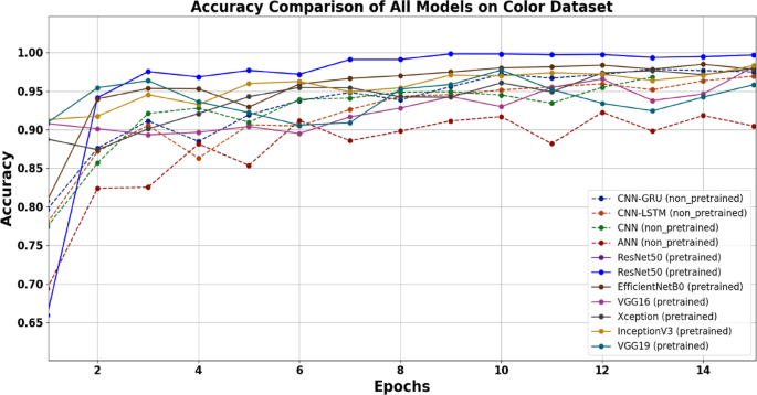
Graph of the accuracy against the epoch across all models (pretrained and non-pretrained). The consistently lowest-performing model is ANN, whereas RsNet50 consistently ranks highest.
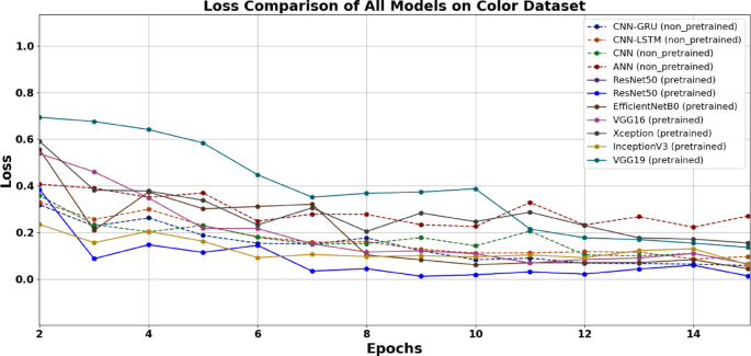
Graph of the loss against the epoch across all models (pretrained and non-pretrained). The consistently lowest loss performing model is ResNet50, whereas ANN shows the highest loss.
Color datasets inherently provide more information through pixel variations, which may help models distinguish between ransomware and benign behaviors. However, the negligible drop in performance across most models when grayscale datasets are used suggests that the essential features for ransomware detection can still be effectively captured with fewer color-specific details.
Robustness and computational efficiency
To assess both detection performance and computational demands, we compared six pretrained CNN models (ResNet50, EfficientNetB0, InceptionV3, Xception, VGG16, and VGG19) with and without fine-tuning. The results, summarized in Table 10, show that fine-tuning generally improved classification accuracy across most models while also reducing training time per sample.
Notably, ResNet50 achieved the highest accuracy improvement from 99.91 to 99.96%, with a reduced training time of 0.440 s/sample (down from 0.571). EfficientNetB0 also demonstrated strong performance with lower training cost. By contrast, models such as VGG16 and VGG19 required more time and showed limited gains, indicating their inefficiency for small datasets.
These results highlight that transfer learning with fine-tuning offers a balanced trade-off, achieving a high detection accuracy while maintaining computational efficiency. Among all the tested models, ResNet50 provided the best combination of speed and robustness for small ransomware datasets.
Model interpretability and visual analysis
To better understand the decision-making behavior of our deep learning models, we conducted a visual interpretability analysis using t-distributed stochastic neighbor embedding (t-SNE) and saliency maps. These methods help reveal how well the model separates ransomware and benign samples in the learned feature space and which regions of the input images most influence classification decisions. By employing these techniques, we aimed to provide deeper insights into the internal representations learned by pretrained CNNs and evaluate the consistency and reliability of the classification outcomes.
t-SNE feature visualization
To enhance the transparency of the model behavior, t-distributed stochastic neighbor embedding (t-SNE) was applied to the final dense layer outputs of the ResNet50 model. As shown in Fig. 8, the ransomware and benign samples are from two distinct clusters, with orange points indicating benign samples and green points representing ransomware.
Although some overlap was observed near the cluster boundary, the overall separation was clear, supporting the model’s high classification accuracy of 99.96%. Rare misclassifications (one false negative) likely occurred in the overlapping region, where a ransomware sample displayed benign-like behavior.
This clustering pattern highlights the ability of the model to map behaviorally distinct classes into well-defined regions in the latent space, thereby reducing the risk of misclassification. Therefore, the rare misclassification observed is explainable and expected in boundary scenarios, further affirming the robustness and reliability of the proposed detection pipeline.
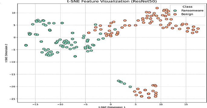
t-SNE feature visualization of used ransomware dataset. Orange points represent benign samples and green points represent ransomware. The two classes formed distinct clusters with limited overlap, illustrating strong feature separability and explaining the near-perfect classification accuracy of the model.
Saliency map interpretation
To gain insight into the internal focus of the model during prediction, we applied saliency mapping using gradient-based backpropagation to the representative samples of both benign (B) and ransomware (R). This technique highlights the most influential pixel regions in the input images, allowing us to interpret which behavioral patterns the model attends to when classifying a sample as ransomware or benign.
As shown in Fig. 9, the saliency maps reveal distinct patterns of attention for the benign and ransomware inputs. For benign samples (left), the focus of the model is limited to a small, dispersed set of pixels, suggesting sparse activation. In contrast, the ransomware (right) saliency map shows intense, localized attention in specific regions, indicating that the model has learned to associate certain behavioral patterns (e.g., registry access and file encryption events) in the presence of the ransomware.
These visualizations demonstrate that the model does not respond to random noise but instead focuses on meaningful regions in the behavioral image. This further reinforces the reliability of the model and its high predictive accuracy of 99.96%.
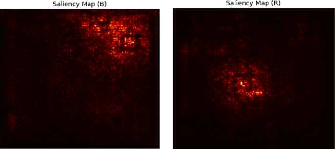
Saliency maps of representative benign (left) and ransomware (right) images. The highlighted regions indicate the pixels with the highest impact on the prediction of the model. The model focuses on structured behavior-encoded areas and confirms the class-specific pattern learning.
Misclassification analysis
To further evaluate the classification performance of the best-performing model, ResNet50, we analyzed its misclassification behavior using a confusion matrix derived from the model weights saved at epoch 24, which corresponded to the highest training accuracy of 99.96%, and evaluated it on the 200-sample validation set (98.50%).
As shown in Fig. 10, the confusion matrix reveals three misclassifications: two false positives (FP) and one false negative (FN), resulting in a validation accuracy of 98.50%. This indicates that two benign samples were incorrectly predicted as ransomware and one ransomware sample was misclassified as benign. These raw counts show the performance of the model, correctly classifying 197 of the 200 validation samples. This matrix reflects the prediction performance of the model at convergence and is generated using the saved model weights after training.
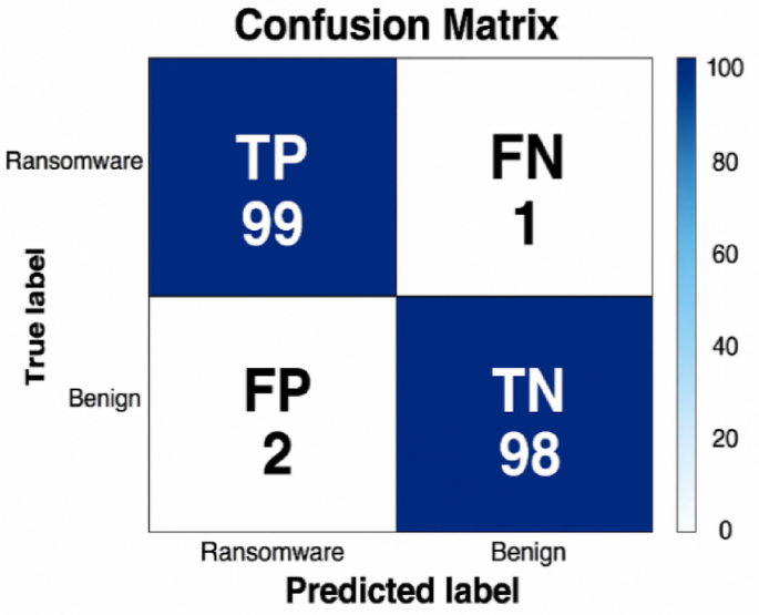
Confusion matrix for the best performing model ResNet50, evaluated on the 200-sample validation set (98.50% accuracy).
Despite these minor errors, the results confirm the high classification accuracy of the model, with near-perfect identification of both benign and ransomware samples. These findings reinforce the effectiveness of the transfer-learning-based model, which maintained a consistently low misclassification rate. These rare errors are likely attributable to borderline case either benign software exhibiting anomaly like behavior or ransomware instances that mimic benign traits to evade detection. This interpretation is supported by the supplementary visualizations such as t-SNE and saliency map. The t-SNE plot revealed distinct clustering between benign and ransomware samples, with minimal overlap, indicating strong feature separability. Furthermore, saliency map analysis demonstrates that the model consistently focuses on behaviorally relevant regions, thereby reinforcing the reliability of its decision-making process.
Overall, the rarity and interpretability of the misclassification patterns confirm the ResNet50-based model’s robustness and generalization capability under transfer learning, even with unseen validation data.
Comparison of our proposed technique with the existing relevant methods
This section compares the performance of the proposed ransomware detection framework with those of several recent approaches, as summarized in Table 11. It is important to note that the studies listed in Table 11 utilized different datasets, feature engineering strategies (e.g., static vs. dynamic), and varying malware types or versions that limited the fairness of direct comparison. While our method is based on a custom dynamic behavioral dataset, most existing approaches rely on static binaries, memory dumps, or hybrid combinations. Thus, the performance results presented in Table 11 are not intended for direct one-to-one comparison but rather to provide contextual benchmarking across a range of related methodologies. Against this benchmark, our proposed method achieved an accuracy of 99.96% on our balanced and threat-informed dataset, thereby demonstrating its effectiveness. To the best of our knowledge, no previous study has utilized this dynamic-to-image transformation technique for ransomware detection, making our approach a novel contribution to the literature.
Several studies have reported competitive results using static analysis. For example16,67, achieved accuracies of 99.50% and 99.20%, respectively, using image-based static features. However, static analysis methods are often more vulnerable to the obfuscation and packing techniques employed by modern ransomware. In contrast, our method incorporates dynamic behavioral data, enabling a more robust detection of evasive threats.
Further comparisons with dynamic and hybrid models using structured input formats (e.g., CSV) also support the strength of our approach. A technique proposed by8,23,24, and28 achieved accuracy scores ranging from 95.90 to 98.20%. Although promising, these results remained below the performance achieved by our framework.
Overall, these findings underscore the advantage of converting structured behavioral data into images, allowing pretrained CNNs such as ResNet50 to exploit spatial patterns and significantly enhance detection performance, particularly in small dataset scenarios.


