Study area and data acquisition
The main objective of this study is to forecast the natural flow pattern of the Nile River at the AHD site, which is located in the southern region of Egypt, as depicted in Fig. 1. The AHD is a large reservoir constructed in southern Egypt by damming the river. Its construction aimed to control flooding, generate hydroelectricity, and provide irrigation water. This study uses natural flow data records spanning 130 years (from 1870 to 2000) at the AHD as the basis for the dataset43. This research utilized the Nile River inflow data from Aswan, as published by the Egyptian Ministry of Water Resources and Irrigation. This dataset is one of the most extensive and long-lasting of its kind, providing valuable insight into the long-term flow trends in the region. The fluctuating flow pattern is clearly depicted in Fig. 2, which illustrates the yearly flow.

The location of the case study Aswan High Dam (AHD).

Natural monthly streamflow of the Nile River in the BCM.
Model Descriptions
In this section, a full description of the proposed algorithms and models is provided. First, a clear representation of the foundation of the proposed algorithms, including the PSS, INFO, and RUN algorithms, is provided. Subsequently, comprehensive discussions of the ELM model for time-series modeling will be reported. Finally, the proposed hybrid model, which combines metaheuristic algorithms and an ELM network, is presented.
Before describing the details of the proposed algorithms, the initialization process, fitness function, and several symbols used throughout the three proposed algorithms are introduced below. All metaheuristic optimization algorithms involve an initialization process. This process starts by initializing N random solutions (population size or pop_size). Each solution is a D-dimensional vector (D variables or problem size) obtained using a uniform random distribution, which can be described by Eq. (1).
$$X_{i,j}^{0} = X_{j}^{min} + R_{i,j} .\left( {X_{j}^{max} – X_{j}^{min} } \right)$$
(1)
where i = 1,2… N; j = 1,2,…. D; \(X_{i,j}^{0}\) is the initial position vector of the \(i^{th}\) solution; \(X_{j}^{min}\) and \(X_{j}^{max}\) denote the minimum and maximum values, respectively, for the \(j^{th}\) dimension of the \(i^{th}\) solution; and \(R_{i,j}\) is a uniform random value in the range of [0, 1].
The fitness function is a function that is used to evaluate the quality of a solution and can be composed of one or multiple objective functions or variations of objective functions. For minimization problems, the lower the fitness function is, the better the solution, and conversely, the higher the fitness function is, the worse the solution. Some of the standard notations used throughout this paper are presented in Table 1.
Pareto-like sequential sampling (PSS) optimization
The PSS algorithm is a recently proposed optimization algorithm35 based on simple sampling and design-of-experiment (DOE) methods, such as Monte Carlo and Latin hypercube sampling. Despite its simplicity, the PSS has been shown to outperform several recent algorithms (PFA, PSO, WOA, etc.) in benchmark functions and engineering problems35. The algorithm starts by initializing a set of N vectors with random coefficient vectors generated using DOE methods as modeled in Eq. (2)
$$X_{i, j} = X_{j}^{min} + R_{i,j} \odot \left( {X_{j}^{max} – X_{j}^{min} } \right)$$
(2)
where \(X_{j}^{min}\) and \(X_{j}^{max}\) are the lower bound and upper bound for the jth dimension, respectively; \(R_{i,j}\) is the random variable generated using the DOE sampling method; and \(\odot\) is the elementwise multiplication of vectors. After the initialization of the population, the PSS algorithm determines the best solution to rescale the lower and upper bounds for the prominent area (Eq. 3), which is then used to update the next positions of the solutions.
$$X_{j}^{min1} = X_{best, j} – \delta_{j} ; X_{j}^{max1} = X_{best, j} + \delta_{j}$$
(3)
$$\delta_{j} = \frac{1}{2}\left( {1 – \alpha } \right)\left( {1 – \frac{g}{{g_{max} }}} \right)\left( {X_{j}^{max} – X_{j}^{min} } \right)$$
(4)
where the acceptance probability α describes the resampling of the 80/20 analogy. After that, the PSS updates the position of the current search agent using either the prominent domain (with the new lower and upper bounds) or the overall domain (the default lower and upper bounds). This process can be modeled using Eqs. (5) and 6
$$X_{i,j}^{g + 1} = X_{j}^{min1} + \mu_{i,j } \odot \left( {X_{j}^{max1} – X_{j}^{min1} } \right)$$
(5)
$$X_{i,j}^{g + 1} = X_{j}^{min} + \mu_{i,j } \odot \left( {X_{j}^{max} – X_{j}^{min} } \right)$$
(6)
where \(\mu_{i,j}\) is a random variable generated using the DOE sampling method and \(\odot\) represents the elementwise multiplication of vectors. The flowchart of the PSS algorithm is shown in Fig. 3.

Pareto-like Sequential Sampling (PSS) Optimization.
Weighted mean of vectors (INFO) optimization
The INFO algorithm is a recent math-inspired metaheuristic proposed by37. It consists of four key phases: initialization (described above), updating rule, vector combining, and local search. Due to its solid mathematical concepts, INFO has been demonstrated to be effective in several applications, such as engineering optimization44, image classification tasks45, and feature selection46. This section briefly overviews some of the main operators and equations used in INFO, with more detailed information available in37.
Updating rule phase
Generally, INFO generates a set of random vectors and then derives the weighted mean from these vectors instead of modifying the position of the current vector toward an optimal solution. The mean rule can be described as follows:
$$MeanRule = r1*WM1^{g} + \left( {1 – r1} \right)*WM2^{g}$$
(7)
$$WMt^{g} = \delta *\frac{{w_{1} \left( {X_{a1} – X_{a2} } \right) + w_{2} \left( {X_{a1} – X_{a3} } \right) + w_{3} \left( {X_{a2} – X_{a3} } \right)}}{{w_{1} + w_{2} + w_{3} + \varepsilon }} + \varepsilon *randn$$
(8)
$$w_{1} = \cos \left( {f\left( {X_{a1} } \right) – f\left( {X_{a2} } \right) + \pi } \right)*{\text{exp}}\left( { – \left| {\frac{{f\left( {X_{a1} } \right) – f\left( {X_{a2} } \right)}}{w}} \right|} \right)$$
(9)
$$w_{2} = \cos \left( {f\left( {X_{a1} } \right) – f\left( {X_{a3} } \right) + \pi } \right)*{\text{exp}}\left( { – \left| {\frac{{f\left( {X_{a1} } \right) – f\left( {X_{a3} } \right)}}{w}} \right|} \right)$$
(10)
$$w_{3} = \cos \left( {f\left( {X_{a2} } \right) – f\left( {X_{a3} } \right) + \pi } \right)*{\text{exp}}\left( { – \left| {\frac{{f\left( {X_{a2} } \right) – f\left( {X_{a3} } \right)}}{w}} \right|} \right)$$
(11)
$$\delta = \left( {2*r2 – 1} \right)*\beta = \left( {2*r2 – 1} \right)*2*{\text{exp}}\left( { – 4* \frac{g}{{g_{max} }}} \right)$$
(12)
where \(g\) and \(g_{max}\) represent the current generation (iteration/epoch) and maximum number of generations, respectively. \(r1\) and \(r2\) are random numbers generated from the ranges [0, 0.5] and [0, 1], respectively. \(randn\) is a random number generated from a normal distribution. \(\varepsilon\) is a very small number, \(f()\) is the fitness function, and \(t\) is the index of the WM. When \(t = 1\), then \(a1, a2\) and \(a3\) are different intergers chosen randomly from the [1, N] range, and \(w = \max \left( {f\left( {X_{a1} } \right), f(X_{a2} } \right), f(X_{a3} ))\). When \(t = 2\), \(X_{a1} = X_{best}\) represents the best solution, \(X_{a2} = X_{better}\) represents the better solution, \(X_{a3} = X_{worst}\) represents the worst solution in the current iteration, and \(w = f\left( {X_{a3} } \right)\). After calculating \(MeanRule\), INFO generates 2 new solutions \(z1\) and \(z2\) based on \(X_{best}\), \(X_{better}\), \(X_{a1}\), and the current solution \(X_{i}\). In the case of a random number \(r3 < 0.5\), \(z1\) and \(z2\) are generated by Eq. (13). Otherwise, \(z1\) and \(z2\) are generated by Eq. (14).
$$\left\{ {\begin{array}{*{20}l} {z1 = X_{i} + \sigma *MeanRule + randn*\frac{{X_{best} – X_{a1} }}{{f\left( {X_{best} } \right) – f\left( {X_{a1} } \right) + 1 }}} \hfill \\ {z2 = X_{best} + \sigma *MeanRule + randn*\frac{{X_{a1} – X_{best} }}{{f\left( {X_{a1} } \right) – f\left( {X_{best} } \right) + 1 }}} \hfill \\ \end{array} } \right.\,\,\,\,\,\,\,if\,\,\,\,r3 < 0.5$$
(13)
$$\left\{ {\begin{array}{*{20}l} {z1 = X_{a1} + \sigma *MeanRule + randn*\frac{{X_{a2} – X_{a3} }}{{f\left( {X_{a2} } \right) – f\left( {X_{a3} } \right) + 1 }}} \hfill \\ {z2 = X_{best} + \sigma *MeanRule + randn*\frac{{X_{a1} – X_{a2} }}{{f\left( {X_{a1} } \right) – f\left( {X_{a2} } \right) + 1 }}} \hfill \\ \end{array} } \right.\,\,\,\,\,\,\,if\,\,\, r3 \ge 0.5$$
(14)
$$\sigma = \left( {2*r4 – 1} \right)*\alpha = \left( {2*r4 – 1} \right)*c*{\text{exp}}\left( { – d*\frac{g}{{g_{max} }}} \right)$$
(15)
where \(c = 2, d = 4\) are two constant numbers and \(r3\) and \(r4\) are random numbers generated from the [0, 1] range.
Vector-combining phase
In this phase, INFO combines two vectors, \(z1\) and \(z2\), to improve diversity. If the random probability is less than 0.5, the new vector will be the same as the current vector. Otherwise, INFO will generate a new vector, as in Eq. (16).
$$X_{i}^{g + 1} = \left\{ {\begin{array}{*{20}l} {X_{i}^{g} ,} \hfill & {if\,\,\, r5 \ge 0.} \hfill \\ {\left\{ {\begin{array}{*{20}c} {z1 + \mu \left| {z1 – z2} \right|, r6 < 0.5} \\ {z2 + \mu \left| {z1 – z2} \right|, r6 \ge 0.5} \\ \end{array} } \right.,} \hfill & {if\,\,\, r5 < 0.5} \hfill \\ \end{array} } \right.$$
(16)
where \(\mu = 0.05*randn\), \(r5\) and \(r6\) are random numbers generated from the (0, 1) range, and \(X_{i}^{g + 1}\) is the new position of the current search agent.
Local search phase
To further enhance the search performance, INFO utilizes a local search strategy around the global best solution and the solution derived from the mean-based rule. This phase is activated for the current agent only when the probability of a randomly generated number is smaller than 0.5. The agent skips this phase if the random probability is greater than or equal to 0.5. The new position of the current solution is presented in Eq. (17).
$$X_{i}^{g + 1} = \left\{ {\begin{array}{*{20}l} {X_{best} + randn*(MeanRule + randn*\left( {X_{best} – X_{a1} } \right), } \hfill & { if\,\,\,\,r7 < 0.5} \hfill \\ {X_{rnd} + randn*(MeanRule + randn*\left( {v_{1} *X_{best} – v_{2} *X_{rnd} } \right),} \hfill & { if\,\,\,\, r7 \ge 0.5} \hfill \\ \end{array} } \right.$$
(17)
$$X_{rnd} = \emptyset *X_{avg} + \left( {1 – \emptyset } \right)*\left( {\emptyset *X_{better} + \left( {1 – \emptyset } \right)*X_{best} } \right)$$
(18)
$$X_{avg} = \frac{{X_{a1} + X_{a2} + X_{a3} }}{3}$$
(19)
$$v1 = \left\{ {\begin{array}{*{20}l} {2*rand,} \hfill & { if\quad r8 > 0.5} \hfill \\ {1,} \hfill & { if\quad r8 \le 0.5} \hfill \\ \end{array} } \right.;\,\,\,v2 = \left\{ {\begin{array}{*{20}l} {2*rand,} \hfill & { if\quad r9 > 0.5} \hfill \\ {1,} \hfill & { if\quad r9 \le 0.5} \hfill \\ \end{array} } \right.$$
(20)
where \(r7, r8\), \(r9\) and \(\emptyset\) are random numbers generated from the (0, 1) range. Finally, the flowchart of the INFO algorithm is presented in Fig. 4.

Weighted mean of vectors (INFO) optimization.
Runge Kutta optimization (RUN)
This section briefly overviews the Runge–Kutta optimization (RUN) algorithm39. The RUN algorithm is based on the Runge‒Kutta method, which is commonly used in numerical methods to solve ordinary differential equations. The RUN algorithm consists of three phases: the first phase is initialization (described above), the second phase involves a search procedure based on the Runge–Kutta theory, and the third phase is enhanced solution quality (ESQ). RUN has the benefit of being simple to execute and effective; therefore, it has been successfully applied in several fields, such as photovoltaic systems47, optimizing hydropower reservoirs40, and feature selection48. The subsequent subsection will briefly describe the RUN algorithm’s main equations and fundamental concepts; more details are available at39.
Search mechanism-based Runge–Kutta theory
In this phase, the RUN algorithm uses a search mechanism (SM) to update the position of the current solution at each generation. It can be determined by Eq. (21).
$$X_{i}^{g + 1} = \left\{ {\begin{array}{*{20}l} {X_{c} + r4*SF*r5*X_{c} + SF*SM + \mu *X_{s1} ,} \hfill & { if\quad pr1 < 0.5} \hfill \\ {X_{m} + r4*SF*r5*X_{m} + SF*SM + \mu *X_{s2} , } \hfill & { if \quad pr1 \ge 0.5} \hfill \\ \end{array} } \right.$$
(21)
$$X_{s1} = randn*\left( {X_{m} – X_{c} } \right);\,\,\,\,X_{s2} = randn*\left( {X_{r1} – X_{r2} } \right)$$
(22)
$$X_{c} = \varphi X_{i} + \left( {1 – \varphi } \right)X_{r1} ;\,\,\,X_{m} = \varphi X_{best} + \left( {1 – \varphi } \right)X_{best}^{g}$$
(23)
$$SF = 2*\left( {0.5 – r6} \right)*f = 2*\left( {0.5 – r6} \right)*a*{\text{exp}}\left( { – b*r7*\frac{g}{{g_{max} }}} \right)$$
(24)
$$SM = \frac{1}{6}X_{rk} *\Delta x = \frac{1}{6}\left( {k_{1} + 2k_{2} + 2k_{3} + k_{4} } \right)*\Delta x$$
(25)
$$k_{1} = \frac{1}{2\Delta x}*\left( {rand*X_{wr}^{g} – u*X_{br}^{g} } \right)$$
(26)
where \(r4\) is a random integer from the set {1,− 1} and \(r5\) is a random number generated from the [0, 2] range. \(pr1\), \(r6\), \(r7\), and \(\varphi\) are random numbers generated from the (0, 1) range. \(a\) and \(b\) are two constant numbers. \(\mu = 0.5 + 0.1*randn\) is a random number. \(X_{wr}^{g}\) and \(X_{br}^{g}\) are the worst random and best random solutions determined based on three random solutions (\(X_{r1} , X_{r2} , X_{r3} )\) selected from the current population with condition \(r1 \ne r2 \ne r3 \ne i\). The rule is defined as follows:
If the fitness of \(X_{i}\) is better than the fitness of the best solution \(X_{bi}\) selected from (\(X_{r1} , X_{r2} , X_{r3} )\), then we have \(X_{wr}^{g} = X_{bi}\) and \(X_{br}^{g} = X_{i}\).
Otherwise, we have \(X_{wr}^{g} = X_{i}\) and \(X_{br}^{g} = X_{bi}\)
$$\Delta x = 2*rand*\left| {rand*\left( {\left( {X_{br}^{g} – rand*X_{avg} } \right) + \gamma } \right)} \right|$$
(27)
$$\gamma = rand*(X_{i} – rand*\left( {X^{max} – X^{min} } \right))*{\text{exp}}\left( { – 4*\frac{g}{{g_{max} }}} \right)$$
(28)
$$k_{2} = \frac{1}{2\Delta x}\left[ {rand*\left( {X_{wr}^{g} + r8*k_{1} *\Delta x} \right) – \left( {u*X_{br}^{g} + r9*k_{1} *\Delta x} \right)} \right]$$
(29)
$$k_{3} = \frac{1}{2\Delta x}*\left[ {rand*\left( {X_{wr}^{g} + r8*\frac{{k_{2} }}{2}*\Delta x} \right) – \left( {u*X_{br}^{g} + r9*\frac{{k_{2} }}{2}*\Delta x} \right)} \right]$$
(30)
$$k_{4} = \frac{1}{2\Delta x}\left[ {rand*\left( {X_{wr}^{g} + r8*k_{3} *\Delta x} \right) – \left( {u*X_{br}^{g} + r9*k_{3} *\Delta x} \right)} \right]$$
(31)
$$X_{avg} = \frac{{X_{r1} + X_{r2} + X_{r3} }}{3}$$
(32)
where \(r8\) and \(r9\) are random numbers generated from the (0, 1) range.
Enhanced solution quality
This phase is implemented in the RUN algorithm to increase the quality of the solutions and avoid local optima in each generation. Additionally, this phase is executed only when the probability of a random number is smaller than 0.5 (\(pr2 < 0.5)\). The mathematical formulation can be described as Eq. 12
$$X_{i2} = \left\{ {\begin{array}{*{20}l} {X_{i1} + r10*w*\left| {X_{i1} – X_{avg} + randn} \right|,} \hfill & { if\quad w < 1.0} \hfill \\ {X_{i1} – X_{avg} + r10*w*\left| {u*X_{i1} – X_{avg} + randn} \right|,} \hfill & { if\quad w \ge 1.0} \hfill \\ \end{array} } \right.$$
(33)
$$w = rand\left( {0, 2} \right)*{\text{exp}}\left( { – c*\frac{g}{{g_{max} }}} \right)$$
(34)
$$X_{i1} = \beta *X_{avg} + \left( {1 – \beta } \right)*X_{best}$$
(35)
where \(\beta\) is a random number generated from the (0, 1) range. \(c = 5*rand\) is a random number. \(r10\) is a random integer chosen from the set {-1, 0, 1}. The \(w\) factor is used to control the exploitation and exploration process in this phase. For \(w \ge 1\) (at early generations), the solution \(X_{i2}\) tends to explore the search space. When \(w < 1\) (at later generations), the solution \(X_{i2}\) tends to exploit around the \(X_{i1}\) position. To enhance the performance of the new solution, the RUN algorithm also utilizes the new operator when the newly generated solution X is not better than the current solution. It can be expressed using Eq. (36).
$$X_{i3} = X_{i2} – r11*X_{i2} + SF*\left( {r12* X_{rk} + v*X_{br}^{g} – X_{i2} } \right)$$
(36)
where \(r11\) and \(r12\) are random numbers in the (0, 1) range and \(v = 2*rand\) is a random number. It is worth noting that the chance to generate \(X_{i3}\) occurs when \(pr3 < w\), where \(pr3\) is a random number in the (0, 1) range. Finally, the flowchart of the RUN algorithm is shown in Fig. 5.

Runge–Kutta optimization (RUN) algorithm.
Extreme learning machine (ELM)
The extreme learning machine (ELM) algorithm was developed to improve the efficiency and speed of single-hidden-layer feedforward networks (SLFNs) without the need for tuning the hidden weights23. Unlike the MLP (ANN or FFNN), which requires an iterative optimization process to determine the hidden weights, the ELM randomly assigns them. The weights between the hidden and output layers are then calculated using the Moore–Penrose inverse method (Fig. 6). ELM is an “extreme” approach because the hidden weights are adjusted only once during training and are randomly assigned33. This enables the ELM to be trained much faster than traditional neural networks and handle large amounts of data with high-dimensional input spaces. ELM has been successfully applied in a variety of fields, including environmental sciences49, time-series forecasting50, and agriculture51.
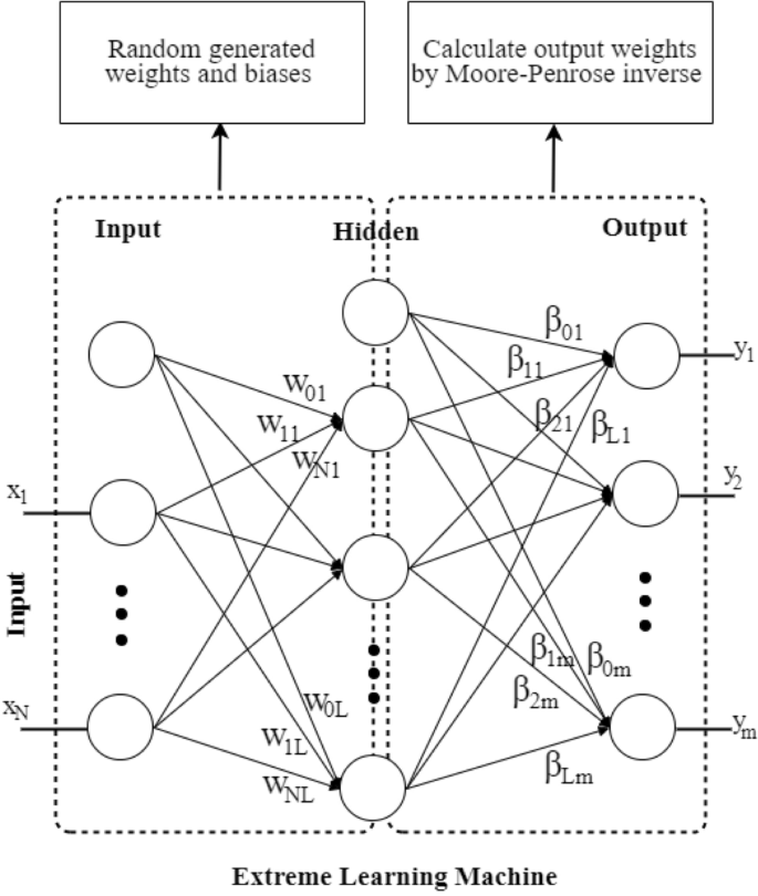
Extreme Learning Machine (ELM).
The most commonly used structure of the ELM is based on an MLP network52 with an input layer, a single hidden layer and an output layer. Given a set of training pairs {\(\left( {x_{i} , y_{i} } \right) \in R^{N}\) x \(R^{m}\)}, where \(x_{i}\) is the input vector with N dimensions and \(y_{i}\) is the m-dimensional output vector, the output of neuron \(j^{th}\) of the ELM with L hidden neurons can be expressed as follows:
$$\hat{y}_{k} = \mathop \sum \limits_{j = 1}^{L} \beta_{kj} .G_{j} \left( {\mathop \sum \limits_{i = 1}^{N} W_{ji} .x_{i} + b_{j} } \right)$$
(37)
where \(G()\) is the activation function and \(W_{ji}\) and \(b_{j}\) are the weights and biases between the input and hidden layers, respectively. \(x_{i}\) is the \(i^{th}\) input node, and \(\beta_{kj}\) is the between hidden and output layers. The training process of ELM is executed as follows:
-
Randomly generated the \(W_{ji}\) and \(b_{j}\)
-
Calculate the \(\beta_{kj}\) by solving least squares problem \(Y = \beta H\), where \(Y\) is the true output (observation values), \(H\) is the output matrix of the hidden layer. \(\beta\) can be calculated using Moore–Penrose inverse which is \(\beta = H^{ + } Y = \left( {H^{T} H} \right)^{ – 1} H^{T} Y\)
Proposed models
Training process of hybrid-based ELM models
Although the ELM employs Moore–Penrose to find the global optimal point for the least squares problem, the matrix H contains random components of the hidden weights. As these weights are generated only once during the training process and are not updated, the use of Moore–Penrose will only locate nonglobal optimal points if the initially generated weights are not globally optimal33. This is the main drawback of the ELM model. Therefore, in this paper, metaheuristic algorithms are proposed to update and find better sets for hidden weights of the ELM network, followed by using Moore–Penrose to calculate the output weights.
Before applying the metaheuristic algorithms, it is essential to define two critical components: the representation of a solution for the optimization problem and the fitness function. These components are addressed for the proposed hybrid-based ELM model (where hybrid-based refers to the proposed algorithms such as PSS, INFO, RUN, and other algorithms that will be compared in the subsequent sections of this study) as follows:
In the proposed hybrid-based ELM model, let \(s_{i} , s_{h}\) and \(s_{o}\) be the sizes of the input, hidden and output layers, respectively. Vectors \(\vec{W}\) and \(\vec{b}\) are the weights and biases of the input and hidden layers, respectively, in the ELM network. A solution is a real vector \(\vec{S}\) (solution), which includes two components: input weights and hidden biases, represented as follows. All values are generated within the range [− 1, 1]:
$$\vec{S} = \left\{ {\vec{W},\vec{b}} \right\} = \left\{ {W_{1,1} \ldots W_{1,L,} W_{N,1} \ldots W_{NL,} ,b_{1} \ldots b_{L} } \right\}$$
All values are generated within the range [− 1, 1]. This vector \(\vec{S}\) encapsulates the necessary parameters for the ELM model, which will be optimized using the proposed metaheuristic algorithms.
In metaheuristic algorithms, the fitness function evaluates the quality of a given solution. In this study, the average root mean square error (\(\overline{RMSE}\)) is selected as the fitness function, a common choice in hybrid-based ELM models. The \(\overline{RMSE}\) is calculated by averaging the RMSE over the entire training dataset, as shown in Eq. (39). In which, Eq. (38) defines the RMSE based on the difference between the ground-truth value and the ELM output.
$$RMSE = \sqrt {\mathop \sum \limits_{i = 1}^{m} \left( {{\hat{\text{y}}}_{i} – y_{i} } \right)^{2} }$$
(38)
$$\overline{RMSE} = \frac{1}{{s_{ts} }}\mathop \sum \limits_{j = 1}^{{s_{ts} }} RMSE_{j} = \frac{1}{{s_{ts} }}\mathop \sum \limits_{j = 1}^{{s_{ts} }} \sqrt {\mathop \sum \limits_{i = 1}^{m} \left( {{\hat{\text{y}}}_{i} – y_{i} } \right)^{2} }$$
(39)
where \(s_{ts}\) denotes the size of the training set, \({\hat{\text{y}}}_{i}\) represents the output of the ELM network (as per Eq. (37)), and \(y_{i}\) represents the corresponding ground truth value.
In this manner, the training process of the ELM network is formulated as an optimization problem aimed at minimizing the RMSE value. Similarly, the hybrid-ELM model can minimize the F(\(\vec{S}\)) = \(\overline{RMSE}\) function. Specifically, the procedure of the proposed hybrid-based ELM models can be described as follows: The proposed algorithm initializes a population of N solutions randomly. Each solution represents a candidate ELM network, as described above. Then, the fitness for each solution is calculated through the following steps:
-
Convert the solution back into input weights and hidden biases, then assign them to the ELM network.
-
Compute the output weights of the ELM using the Pseudo-Inverse Method based on the training dataset.
-
Evaluate the \(\overline{RMSE}\) value based on the validation part of the dataset.
After calculating the \(\overline{RMSE}\) value, it is returned to the fitness function of the metaheuristic algorithms. The algorithms then perform the operation steps described in the earlier sections to evolve the population. This process repeats iteratively until the stopping condition of the algorithm is met. At this point, the solution with the best performance (i.e., the lowest \(\overline{RMSE}\)) is returned to the ELM network. Consequently, we obtain the optimal and most effective ELM model.
Proposed hybrid-based ELM
This section provides a detailed description of our proposed model, illustrated in Fig. 7. Our model consists of two main components: Data Preparation and Modeling (Training and Testing).

Metaheuristic-based ELM Model.
The Data Preparation component aims to collect and prepare data for the model. During the data collection phase, the Data Collection component stores data on servers and retrieves it in CSV format using SQL queries. These CSV files are then passed through the Data Preprocessing component for cleaning and preparation for the model. To use time-series data for machine learning models (i.e. neural network), the first step is to transform it to a supervised learning format using the sliding windows method. The sliding window’s width represents the time series’ lag values. Next, we implement the ANOVA F-test53 to determine the model’s appropriate input variables (best lagged features). This approach is widely employed in hydrology-related domains29,54. According to the findings of the ANOVA F-test, six lagged times are chosen as input features for one-step ahead river streamflow modeling as shown in Table 2.
where Q
Source link