Ethics statement
The UKB study was conducted with the approval of the North-West Research Ethics Committee (ref 06/MRE08/65), in accordance with the principles of the Declaration of Helsinki; all study participants gave written informed consent and were free to withdraw at any time47. This project used data from the UKB study under approved project numbers 53144, 49978 and 11350. All retinal images shown in this paper are reproduced with the permission of UKB.
Cohort characteristics
UKB is a prospective population-based study of 502,355 participants. Baseline examinations were carried out at 22 study assessment centers between January 2006 and October 2010. Study participants have undergone a detailed assessment of demographic, lifestyle and clinical measures; provided DNA samples via blood tests; and provided a range of physical measures. A substantial subset of volunteers underwent an ophthalmic assessment (23%, n = 117,279). Of these participants, 67,664 underwent spectral domain OCT between 2006 and 2010 (‘instance 0’) and an additional 17,090 participants were imaged for the first time during the first repeat assessment between 2012 and 2013 (‘instance 1’)48. UKB data are organized into data categories and fields, and we provide data category and field ID numbers in brackets for reproducibility. The characteristics of those with and without imaging were compared using the Kruskal–Wallis and χ2 tests.
Imaging quality control
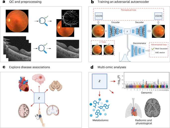
Low-quality OCT scans were excluded on the basis of an image quality score below 40 (ref. 15). The quality score used was that which is native to the Topcon OCT device. CFPs were excluded if they were of ‘reject’ quality grading assessed using a deep learning method, ‘Automorph’ (‘usable’ and ‘good’ images were retained)49. Automorph was trained using the EyePACS-Q dataset, using grading provided by two experts according to image illumination, artifacts and diagnosability of ocular diseases; the full method is documented in the referenced publication.
Image preprocessing
For OCTs, FDS files were converted to an analyzable format using the oct-converter python package50. OCT slice 64 was retained for analysis. CFPs were cropped and segmented using Automorph, and the binary vasculature segmented images were retained for the purpose of refining the autoencoder loss function defined below. Imaging data were randomly split approximately 70:15:15 into train:test:validate allocations for the purpose of training deep learning models. Images were partitioned so that each study participant’s scans were paired within the same allocation.
Autoencoder model architecture and training
Image transformations
Several transformations were applied to OCTs and CFPs during the autoencoder training process. To reduce computational burden, images were resized to 224 × 224 using bicubic interpolation. To improve model generalizability, several further transformations were applied during training, namely, random horizontal flips, random rotations (0–15°), random color jitter (brightness = 0.9–1.1, contrast = 0.9–1.1, saturation = 0.9–1.1).
Model architecture
We designed an AAE for the purpose of creating compressed representations of retinal images (CFP and OCT). The AAE architecture is regularized by matching the aggregated posterior, q(z), to an arbitrary prior, p(z). We selected a Gaussian prior N(0,1), and the resulting vector (z) approximates a multivariate Gaussian distribution51. This property is beneficial for downstream analyses, many of which have a normality assumption. Our AAE was trained in a laterality agnostic manner, but separate AAEs were trained for OCTs and CFPs. The model encoder consisted of each layer of the encoder consisting of a 2D convolution, a batch normalization layer, a Leaky Rectified Linear Unit (ReLU), a multi-scale residual block (kernel sizes 3 and 5) and an efficient multi-scale attention module52,53. We projected our image to a 256-dimensional vector using a linear layer at the bottleneck. Our decoder consisted of a single linear layer for up sampling our vector, followed by 2D transposed convolutions, batch normalization, Leaky ReLU activations, multi-scale residual blocks and efficient multi-scale attention modules52,53. Our adversarial discriminator was composed of three linear layers and used Leaky ReLU activation functions.
Loss functions
For training both the OCT- and CFP-AAE, we used the mean absolute error (also known as L1 loss) and adversarial loss. CFPs are relatively low contrast images, which are dominated by a narrow background color distribution (the retina). For our purposes, the retinal vasculature is an important structure that must be represented in the latent space. In our first iterations of training our model, the AAE failed to reconstruct the vasculature to an acceptable extent, owing to the vasculature contributing little to the L1 loss (for example, Supplementary Fig. 90). Using Automorph, we segmented the CFP images and produced binary masks of the vasculature49. On average, the vasculature represented just 4.07% of the pixels in CFPs. Accordingly, for the CFP-AAE, we weighted the L1 loss to attribute 12.29× more weight to pixels containing blood vessels on Automorph binary masks. In doing so, CFP vasculature structures then contributed 50% of the L1 Loss on average. In addition, we implemented a perceptual loss function for the CFP-AAE. In a previous systematic comparison of deep perceptual loss functions, the 4th ReLU of VGG16 (without batch normalization) was shown to contribute to the best performance in autoencoding tasks, and, accordingly, this model was selected for our perceptual loss function54. To calculate a perceptual loss, original images and AAE reconstructions were normalized according to ImageNet parameters before being passed to VGG16 without batch normalization55. The mean squared error loss of the feature maps of the reconstructed and original images then served as the perceptual loss. Finally, with a view to normalizing the latent vectors produced by the model, we used an adversarial loss function. Briefly, this was calculated by training a discriminator network to distinguish between the latent vectors of the AAE model and a standard normal distribution. To improve the stability of the adversarial network, we used one-sided label smoothing56. The weight provided to each constituent of the loss function was determined using a Bayesian hyperparameter sweep as described below. In our CFP-AAE, terminal arterioles and venules were lost in reconstruction. Although we identified that the SSIM improved with expansion of the latent space (for example, 128-dimensional vectors resulted in an SSIM of 0.876, and 256-dimensional vectors in 0.891), in the interest of preserving the statistical and computational feasibility of downstream tasks, we did not expand the latent space dimensionality further in the pursuit of terminal vascular reconstruction.
Image quality metrics
Image quality metrics used included the PSNR, SSIM and the L1 loss57.
Hyperparameter search
We performed a Bayesian hyperparameter sweep using the Weights and Biases platform (version 0.19.8)58. The SSIM in the test dataset guided the Bayesian optimization. For both CFP and OCT AAEs, the search was used to select the discriminator learning rate, the autoencoder learning rate, the number of convolutional layers, the optimizer weight decay and the weighting of the adversarial loss. For the CFP sweep, we additionally included the perceptual loss weighting. The sweep was conducted for 35 epochs per hyperparameter combination. For the CFP-AAE, the sweep-identified optimal hyperparameters included 5 convolutional layers, a weight decay of 0.01 (AdamW optimizer), an autoencoder learning rate of 0.0005, a discriminator learning rate of 0.0001, a weighting of 0.2 for the perceptual loss and a weighting of 0.001 to the discriminator loss59. For the OCT-AAE, the optimal hyperparameters included 4 convolutional layers, a weight decay of 0.001 (AdamW optimizer), an autoencoder learning rate of 0.0001, a discriminator learning rate of 0.00005 and a weighting of 0.0001 for the discriminator loss.
Additional AAE experimental details
Experiments were conducted using PyTorch60. We used a learning rate to warm up over the first 15 epochs. The batch size was 32. A random seed of value 42 was used. The CFP model was trained for 400 epochs, and the OCT model was trained for 250. For sensitivity analysis, we trained a second OCT and CFP model with 128 dimensions, using the same hyperparameters as those used in our main analysis. Our models were trained using 4 tesla T4 graphics processing units (GPUs). Randomly selected reconstructions were examined by two ophthalmologists (T.H.J. and P.I.S.) to ensure that critical structures were adequately represented in reconstructed images.
OCT- and CFP-AAE phenotypic association tests
We used latent vectors representing the left eye (OCT and CFP) of UKB study participants as a means of reducing the dimensionality of the analysis. In keeping with previous work, the left eye was selected because the relevant images are systematically of higher quality than those from the right eye11,15. The total number of study participants varied according to the requirements of the association test, and are reported in text where possible, or in the supplementary content in which the study participant number varied according to individual phenotype. Both instance 0 and 1 ophthalmic images were used in these analyses (except where explicitly stated otherwise), and where a study participant had undergone imaging during both instances, only their first set of images were considered.
Pearson correlation analyses
The ‘positive control’ Pearson correlation analyses included all traits in the UKB eye measures category (category 100013), excluding right eye measures.
The experimental tests featured a combination of anatomical and functional cardiovascular and neurological traits. Specifically, this featured all traits in the following UKB catalogs: brain MRI (category 1014), cognitive function (category 1005), heart MRI (category 1015) carotid ultrasound (category 101) and selected traits from the physical measures category (category 1006). There was a total of 50 cardiovascular traits and 892 neurological traits. The large number of neurological traits reflects the scale of derived neuroimaging features available in UKB. To enhance theme-wise interpretability in plots, we used HDBSCAN clustering61. Traits present in an overlapping, large number of study participants were clustered, and the remainder of the traits were assigned to a ‘not clustered’ category—but were still considered in subsequent analyses. Data were scaled according to the interquartile range using ‘RobustScaler’ in SciKit Learn62. Clusterable features included 35 ophthalmic traits (n = 62,729), 889 neurological features (n = 12,219) and 37 cardiovascular traits (n = 11,295). A leaf clustering method was used. Cardiovascular and ophthalmic traits were fewer in number, so a minimum cluster size of 3 was used. Neurological traits were assigned a minimum cluster size of 10 given the larger number of traits.
For each analysis, outlier cardiovascular, neurological or ophthalmic values were excluded. This was achieved by excluding data greater than 2.5 standard deviations from the mean. Pearson correlation coefficients and accompanying P values were then calculated using the SciPy python package63.
Cox proportional hazards and Welch’s t-test analyses
Disease outcomes were derived from the ‘First Occurrences’ UKB catalog (category 1712). The UKB first occurrences were generated by mapping read code information in the ‘Primary Care data’ (category 3000), ICD-9 and ICD-10 codes in the ‘Hospital inpatient data’ (category 2000), ICD-10 codes in ‘Death Register records’ (field 40001, field 40002) and ‘self-reported medical condition codes’ (field 20002) reported at the baseline or subsequent UKB assessment center visit. The UKB estimates that hospital inpatient data and death are mostly complete up to 31 May 2022, after which data may be incomplete64. Accordingly, we used 31 May 2022 as the censoring date for our time-to-event analysis. For the Cox proportional hazards, study participants who suffered a given disease event before the date of retinal imaging were excluded from analysis. Meanwhile, for our t-test, the objective was to determine whether latent features differed significantly according to the presence and absence of disease at the time of scan, and so, for this analysis, those with disease events at the time of scan were included. Disease outcomes included (1) a positive control disease dataset inclusive of diseases that were determined to be identifiable on retinal imaging according to two ophthalmologists (T.H.J. and P.I.S.), including disorders of the retina, choroid, optic nerve and lens (19 diseases); (2) all available neurodegenerative diseases (10 diseases); and (3) all available cardiovascular disorders (23 diseases). The complete list of diseases considered is presented in Supplementary Table 31.
Cox proportional hazards modeling was conducted using the lifelines Python package65. The primary outcome of interest was the relationship between left eye Ret-AAE embeddings and time-to-event analyses against ophthalmic, cardiovascular and neurodegenerative diseases. Covariates included genetic sex and age at the time of scan. t-tests were conducted using the SciPy package in Python63. We elected to use the Welch’s t-test, a modification of the Student’s t-test, which is more reliable in the context of unequal sample sizes of variances between two populations66. Results with fewer than 30 samples per group were excluded from the final analysis in both analyses. We were unable to test the baseline relationship between Ret-AAE embeddings and Huntington’s disease, spinal muscular atrophy and related syndromes, Alzheimer’s disease and vascular dementia owing to insufficient cases (<30) at baseline imaging. Huntington’s disease was additionally excluded from Cox proportional hazards analysis owing to insufficient cases.
CCA
CCA was used to explore the relationship between CFP–OCT-derived embeddings and 251 metabolic biomarkers generated by Nightingale Health (category 220)67. Owing to study participant overlap in instance 0 and 1 metabolic sampling, only instance 0 data were used in this analysis. Study participants with missing imaging or missing metabolite samples were excluded. Extreme values that may unduly influence the results were managed using Winsorization (applied to the most extreme upper and lower 1% of values)68. The analysis was conducted using the SciKit learn CCA model. Embeddings and metabolomic data were scaled using the native CCA scaler. To assess the statistical significance of each canonical variate, we used permutation testing to create a null distribution of correlations. The embedding matrices were held constant, while the metabolomic matrix was substituted for randomly permuted sequences over 1,000 iterations69,70. The P value was calculated using the number of null correlations that exceeded the average CCA estimated on the original dataset. The number of modes to test in our permutation test was determined by constructing a Scree plot of the first 10 modes and then truncating where there is a substantial reduction to the regression coefficient.
SPLS
In addition to CCA, we explored metabolomic data using a canonical SPLS analysis using the mixOmics (version 6.32.0) R library71. SPLS is a variant of partial least squares in which a subset of important features is selected for inclusion in the model according to sparsity hyperparameters, rather than including all traits, which may be inappropriate in the context of highly correlated covariates (as is the case for metabolomic data). SPLS was therefore implemented as a means of validating our CCA results in a manner more robust to the structure of our data. Data were prepared in line with the CCA analysis. Lasso penalization was optimized using fivefold cross-validation with five repeats, optimized to maximize correlation between predicted and actual components. Following this, we implemented CFP SPLS with 2 components, 30 embedding variables in component 1 and 10 in component 2, and 25 metabolite variables in component 1 and 10 in component 2. OCT SPLS was implemented with 1 component, with 10 embedding variables and 10 metabolite variables. The analysis was undertaken using the canonical mode, and plots presented with respect to SPLS were all generated using mixOmics.
Genetic analyses
Choice of GWAS method
REGENIE version 4.1 was selected as the method for GWAS72. For step 1, we used the UKB microarray data (field 22418). For step 2, we used the imputed data (field 22828).
Phenotypes and covariate data
The phenotypes studied were latent features for each study participant’s left eye OCT and CFP images. Therefore, 256 GWAS studies were performed per study participant per scan type (that is, 512 GWAS studies in total). Covariates for GWAS were sex (field 31), age at date of scan (field 22006) and spherical equivalent refractive error. Spherical equivalent refractive error was calculated by identifying the most reliable refractometry result (field 5276), identifying the spherical refractive error (field 5085) and cylindrical refractive error (field 5086), and performing the calculation: spherical equivalent = spherical refractive error + 0.5 × cylindrical refractive error15.
Quality control for genetic analyses
The genetic analyses in the discovery cohort were conducted in study participants in instance 0 (initial assessment visit, 2006–2010). The genetic analyses in the replication cohort were conducted in study particpants who attended within instance 1 (first repeat assessment visit, 2012–2013). Any overlapping study participants were removed (that is, the cohorts are entirely independent). Analysis was limited to study participants of genetically determined European ancestry according to their principal components (field 22006).
Study-participant-level genetic quality control metrics were applied, including exclusion of participants whose genetic sex (field 22001) did not match their reported sex (field 31), exclusion of participants with sex chromosome aneuploidy (field 22019), exclusion of participants with genetic kinship to other UKB participants (field 2202), exclusion of participants who were outliers for heterozygosity or missing rate (field 22027) and removal of individuals with more than 10% missing genotype data73.
Variant-level quality control was conducted using plink2 (ref. 74). For the microarray data used in REGENIE step 1, quality control included minimum minor allele frequency of 0.01, minimum minor allele count of 20, removal of variants with >10% missingness and removal of SNPs failing the Hardy–Weinberg equilibrium test at P < 1 × 10⁻¹⁵. For imputed data used in step 2, quality control included minimum minor allele frequency of 0.01, minimum minor allele count of 20, removal of variants with >10% missingness, removal of SNPs failing the Hardy–Weinberg equilibrium test at P < 1 × 10⁻⁶ and removal of duplicate variants. In addition, following GWAS, any variants with an imputed information (INFO) score below 0.8 were removed.
GCTA COJO
To refine the obtained association signals, further analyses were performed using GCTA-COJO12. Genetic variants in loci that were on different chromosomes or more than 1,500 kb distant from each other were assumed to be uncorrelated. Otherwise, GCTA COJO default parameters were implemented.
Gene set analysis
Gene set analysis was performed using MAGMA24. Gene sets were derived from the Human MSigDB Collections75. Specifically, we elected to use the canonical pathways from the curated gene sets. The canonical pathways include the BioCarta pathways database (292 gene sets), the KEGG MEDICUS pathway database (658 gene sets), the PID pathway database (196 gene sets), the Reactome pathway database (1,787 gene sets), the WikiPathways pathway database (885 gene sets) and the KEGG (legacy) pathway database (186 gene sets). Variants were annotated to genes based on dbSNP version 135 variant locations and NCBI 37.3 gene definitions. The LD reference file was derived from the ‘European’ subset of the 1000 Genomes Project dataset76.
Global genetic correlation analysis
The global genetic correlation between OCT and CFP latent features and cardiovascular and neurological disease was assessed using LD score regression (LDSC)77. The GWAS summary statistics for cardiovascular and neurological disease were sourced from publicly available studies in the same genome build used in this study (GRCh37) and containing the required information for genetic correlation78,79,80,81,82,83. Only latent features with a mean chi2 > 1.02 were considered for LD score regression (the threshold for polygenicity). Our analysis was consistent with the methodology outlined in a previous study77, in which genetic variants were filtered according to presence in HapMap3, minor allele frequency > 0.01, INFO score > 0.9 and removal of strand-ambiguous variants and duplicated variants. LD scores were derived from the European subset of the 1000 Genomes Project dataset76. The intercept was not constrained in this analysis. LD score regression was also used to determine the heritability of the polygenic latent features, but not an estimate of statistical significance is not available as this is not an output of the LDSC method.
Grad-CAM
To enhance the interpretability of our learned embeddings, we applied Grad‑CAM84. Consistent with previous work, we observed that visualizations from the earliest convolutional layers lacked semantic relevance, whereas those from the deepest layers were overly coarse to localize meaningful image features85. Consequently, we focused our primary analyses on the third convolutional layer for both CFP and OCT modalities, which provided the optimal balance between spatial resolution and semantic content. In instances in which Grad‑CAM failed to yield an interpretable map, we instead used Layer‑CAM or, alternatively, targeted adjacent convolutional layers; these exceptions are clearly noted in each figure legend86. Saliency maps are only presented for embeddings that are referenced in text. Where possible, we describe embeddings with respect to their anatomical localization to enhance interpretability. Given the abstract nature of embeddings, this is not possible in all cases.
Latent feature traversals
In addition to Grad-CAM, we performed systematic latent feature traversals of the trained AAE87. For each latent dimension (embedding) zi, we first identified a representative reference image whose latent coordinate in that dimension was closest to the mean (that is, approximately zero). This reference latent vector was then held fixed except for zi, which was perturbed independently by ±4 standard deviations. The modified latent vectors were decoded using the AAE decoder to visualize the effect of isolated variation along each latent axis on the reconstructed image.
Because the resulting changes can be visually subtle, we complemented qualitative inspection with quantitative difference maps. For CFPs (three-channel RGB images), we computed the mean change in pixel intensity per color channel relative to the reference reconstruction. For OCT images (single-channel), we computed the absolute per-pixel intensity difference. These visualizations highlight regions most sensitive to variation in each latent dimension and facilitate interpretation of the image features encoded by the learned representation.
The power of autoencoding for feature extraction is that image patterns can be identified that are not necessarily visually apparent to the human eye. Accordingly, many latent traversals result in diffuse pixel intensity changes that are challenging to interpret biologically and clinically. Only figures with human-interpretable features are presented in (Supplementary Figs. 14–68).
Annotations of latent traversals and Grad-CAM saliency maps were provided following independent review by two ophthalmologists (T.H.J. and P.I.S.).
Controlling for type 1 error risk
We elected to implement family-wise error rate control (Bonferroni-corrected threshold for significance) in this analysis. We examined whether autoencoder embeddings were substantially correlated to guide our definition of a family. As can be seen in Supplementary Figs. 91 and 92, the embeddings showed little meaningful correlation. Accordingly, each embedding was treated as its own family, and multiple testing correction was applied according to the total number of tests within each embedding. Given that this is not a study-wide correction (that is, we do not also correct according to the number of embeddings, which would be prohibitively strict and cause excessive type 2 error given the study scale and hypothesis-free nature of this work), we assess our results and the risk of type 1 error in the context of the convergent evidence presented across analyses, present raw P values to allow interpretation by readers, interpret results in the context of their biological plausibility and, where possible, validate results in a separate UKB instance. Although this approach offers a more nuanced perspective on the results, type 1 error remains an area of concern, and the key study findings will benefit from external experimental validation when appropriate external multi-omic datasets become available. The Bonferroni-corrected P value thresholds for significance for all other analyses are presented in the appropriate supplementary table legends.
Statistics and reproducibility
All methodological approaches are described in the relevant sections of the paper. Sample sizes varied by analysis and are reported alongside each result where possible or otherwise provided in the Supplementary Data. No statistical methods were used to predetermine sample size. Instead, all available data passing analysis-specific quality control criteria were included. All analyses were performed using reproducible computational pipelines, as described in the Methods.
Reporting summary
Further information on research design is available in the Nature Portfolio Reporting Summary linked to this article.


