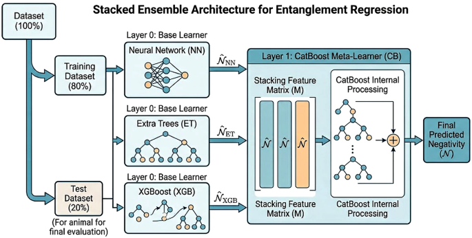
This section presents a comprehensive analysis of the ensemble ML model’s performance in predicting entanglement, specifically the negativity, for multi-spin quantum systems. The ensemble architecture is a stacking model that amalgamates predictions from three diverse base learners: a NN, ET, and XGB. The predictions from these base models are then used as input features for a higher-level meta-learner, CB, which produces the final output. This stacking strategy is designed to capitalize on the distinct strengths inherent to each constituent model. The meta-learner’s task is to learn the optimal way to combine the base predictions, effectively weighting their contributions based on their performance across the problem space, rather than relying on a simple average or manual weighting. The tree-based methods (ET and XGB) complement the NN by enhancing robustness and providing alternative perspectives on feature importance, while the NN excels at capturing complex, non-linear interdependencies within the data. The rationale for this ensemble construction is further discussed in supplemental material. This ensemble approach aims to strike a balance between the representational flexibility of deep learning and the interpretative stability often associated with ensemble tree models, thereby fostering improved predictive accuracy for the regression tasks under investigation.
Robustness of data generation
The primary training dataset was assembled with a stratified sampling strategy in which approximately \(10\%\) of states carry non-negligible negativity, counteracting the concentration of the orthogonal-ensemble Haar measure near \(\mathcal {N} = 0\). To assess whether the model has learned the physical structure of the negativity measure or has instead exploited sparsity artefacts of this specific dataset, performance was evaluated across three generation regimes shown in Figure 2.

Negativity distributions \(P(\mathcal {N})\) at \(J = 1\). Main figure (blue): training distribution; red insets: held-out test distribution. (a) Structured: \(10\%\) of states have \(\mathcal {N}>0\), \(20\%\) of \(C_{mn}\) entries set to zero (\(R^{2}=0.9962, \hbox {MSE}=5.6\times 10^{-3}, \hbox {MAE}=0.054\)). (b) Semi-structured: no forced entanglement, \(20\%\) random zero entries (\(R^{2}=0.9748\), \(\hbox {MSE}=7.7 \times {10}^{-2}\), \(\hbox {MAE}=0.143\)). (c) Unstructured: purely random Gaussian-Haar sampling (\(R^{2}=0.9519\), \(\hbox {MSE}=0.162\), \(\hbox {MAE}=0.243\)).
The ensemble was trained on regime (a) and applied without retraining to regimes (b) and (c). On the training distribution, \(R^{2}=0.9962\) and \(\textrm{MSE}=5.6\times 10^{-3}\). Generalisation to the semi-structured regime (b) gives \(R^{2}=0.9748\) and \(\textrm{MSE}=7.7\times 10^{-2}\), and to the fully unstructured regime (c), \(R^{2}=0.9519\) and \(\textrm{MSE}=0.162\). The progressive decrease in \(R^{2}\) from (a) to (c) reflects the growing statistical distance between the test and training distributions, not a breakdown of the learned mapping. Retaining \(R^{2}>0.95\) under this distributional shift indicates that the ensemble has captured invariant features of the negativity measure rather than sparsity patterns specific to regime (a).
Statistical robustness and seed-averaged performance
To verify that the reported metrics are not an artefact of a particular random initialisation or data split, the entire pipeline—Gaussian-Haar state generation, base-learner training, and meta-learner fitting—was repeated for five independent random seeds (42, 123, 456, 789, and 1024).
Tables 1 and 2 summarise the resulting metrics for pure and Werner states at \(J = 1/2, 1\), and 5. Across all dimensions the standard deviation of \(R^{2}\) does not exceed 0.0006, and those of MSE and (Mean Absolute Error) MAE are similarly negligible, confirming that the stacking architecture provides stable predictions independently of stochastic initialisation.
To characterise the computational cost of the framework, we recorded the average training time and peak memory usage across the five runs; the results are given in Table 3.
Both quantities grow super-linearly with J. Between \(J=1\) and \(J=5\) the memory footprint increases by \(321\%\) and the training time by a factor of 3.6, consistent with the expansion of the Werner-state feature vector, whose length scales as \((2J+1)^{4}\). Within the investigated range a simple regression yields the empirical estimates
$$\begin{aligned} T(J) \approx 44.78\,J + 17.40 \quad (\text {s}), \qquad M(J) \approx 3.02\,J^{2} – 3.87\,J + 18.61 \quad (\text {MB}), \end{aligned}$$
(12)
where the linear form for T and the quadratic form for M are empirical fits valid for \(J \le 5\); extrapolation beyond this range should be treated with caution given the limited number of data points. For \(J \le 5\) the resource requirements are modest on standard workstation hardware, but the trends in Eq. (12) identify a potential scalability ceiling for raw density-matrix flattening at larger spin dimensions. Alternative input representations, such as descriptors derived from the quantum Fisher information matrix, will be explored in future work to mitigate the \((2J+1)^{4}\) growth of the feature space.
Performance scaling with dataset size and derivation of an empirical formula
A critical aspect of evaluating any ML model is understanding its performance scalability with respect to the volume of training data, particularly when addressing problems like entanglement quantification that suffer from the ”computational bottleneck” inherent in high-dimensional quantum systems. Figure 3 provides a detailed examination of this relationship for the ensemble model when applied to pure quantum states, across varying spin dimensions characterized by \(J = 0.5, 1,\) and 5. The analysis focuses on three standard performance metrics: MSE, MAE, and the coefficient of determination (\(R^2\)).

Pure state metrics with respect to the number of random states in the case of pure states.
As anticipated from established ML principles, the results consistently demonstrate that increasing the number of training samples leads to an enhancement in model performance across all considered spin values. This is manifested by a monotonic decrease in both MSE (Fig. 3, top figure) and MAE (Fig. 3, middle figure), coupled with a corresponding monotonic increase in the \(R^2\) score (Fig. 3, bottom figure), as the sample size (plotted on a logarithmic x-axis) expands. This trend underscores the model’s ability to learn underlying patterns more effectively and generalize better when provided with more extensive training data.
A salient observation is the pronounced dependence of convergence speed and ultimate performance on the dimensionality of the quantum system, represented by the spin quantum number J. For lower-dimensional systems (e.g., \(J = 0.5\), indicated by red circles), the model exhibits rapid performance improvements. Error metrics decrease sharply, and the \(R^2\) value swiftly approaches unity, indicating near-optimal performance achieved with a relatively modest number of samples (on the order of \(10^3\)). The \(J = 1\) system (blue squares) follows a similar trajectory but necessitates a moderately larger dataset to attain comparable levels of accuracy.
In stark contrast, the high-dimensional \(J = 5\) system (black triangles) demonstrates significantly slower convergence. The MSE and MAE decrease more gradually, and the \(R^2\) score ascends at a much-reduced rate. This signifies a substantially greater data requirement to achieve high-fidelity entanglement predictions for higher-spin systems. This behavior is intrinsically linked to the exponential growth of the Hilbert space dimension with J, leading to a vastly more complex state space and entanglement landscape that the model must learn to navigate. Even at the maximum depicted sample size of \(10^5\), the \(R^2\) for \(J = 5\) is still visibly improving and has not yet reached an asymptotic performance level, unlike the curves for \(J = 0.5\) and \(J = 1\), which exhibit saturation or diminishing returns at smaller sample sizes. This highlights the ”curse of dimensionality” impacting the data efficiency of the learning process.

Werner states metrics with respect to the number of random states in the case of Werner states.
Figure 4 extends this scalability analysis to Werner states, which serve as a proxy for more realistic mixed quantum systems incorporating noise and statistical mixtures. The plots again illustrate MSE, MAE, and \(R^2\) as functions of training sample size (logarithmic scale) for spin dimensions \(J = 0.5, 1,\) and 5. Consistent with observations for pure states, increasing the sample size invariably leads to improved predictive accuracy across all dimensions. Both MSE and MAE exhibit a clear downward trend, while \(R^2\) correspondingly increases.
The rate of performance improvement for Werner states is also strongly contingent on the system’s dimensionality (J). The \(J = 0.5\) system (red circles) demonstrates the most rapid convergence. The \(J = 1\) system (blue squares) requires a larger dataset (approximately \(10^4\) samples) to reach comparable saturation levels. The high-dimensional \(J=5\) case (black triangles) presents a considerably greater challenge, with its convergence being markedly slower. The increased complexity arising from mixedness, compounded by higher dimensionality, means that even at \(10^5\) samples, the \(R^2\) for \(J = 5\) (while high at nearly 0.98) appears to be still ascending, suggesting that optimal characterization of entanglement in such high-dimensional mixed states might demand even larger datasets.
Overall, Figs. 3 and 4 confirm the ensemble model’s robustness in handling both pure and mixed quantum states. They underscore that while the ML approach shifts the computational burden from direct calculation on individual states to data generation and model training, the training data requirement itself scales significantly with system complexity. This empirically justifies the strategic use of progressively larger datasets for higher J values.
Leveraging these observed performance trends, we sought to derive a phenomenological scaling law to estimate the number of training samples (S) required. A linear regression model was applied to the aggregated data from Figs. 3 and 4, using performance metrics (MSE, MAE, \(R^2\)) and the spin quantum number J as input features, with \(\log _{10}(S)\) as the target variable. This analysis yielded the following empirical relationship
$$\begin{aligned} \log _{10}(S) \approx 2.8 + (0.502)\ J – (3.042) \ \text {MSE} – (8.012) \ \text {MAE} + (1.012)\ R^2. \end{aligned}$$
(13)
This heuristic formula provides a quantitative guideline for estimating data requirements. The positive coefficient for J (+0.502) quantitatively confirms that the necessary sample size S grows exponentially with the spin quantum number, as expected from the ”curse of dimensionality.” It is insightful to consider this scaling in the context of the Hilbert space dimension, \(D = (2J+1)^2\). The logarithm of the number of samples, \(\log _{10}(S)\), appears to scale roughly linearly with J. This empirical finding suggests that the complexity of the learning task, while substantial, may not scale directly with the full state space dimension (which would be closer to \(\log (D) \approx 2\log (2J+1)\) for large J), but rather with a simpler proxy for its complexity. The signs of the other coefficients are also intuitive: achieving lower errors (MSE, MAE) requires more samples, hence the negative coefficients for these terms, while achieving a higher coefficient of determination (\(R^2\)) also requires more samples, as indicated by its positive coefficient. While this formula is an empirical approximation specific to our ensemble architecture and dataset characteristics and should be applied cautiously outside the investigated parameter range, it offers a practical tool for initial resource estimation in similar studies. The dataset sizes employed elsewhere in this study (e.g., \(10^4\) for \(J=0.5\), \(2 \times 10^4\) for \(J=1\), and \(10^5\) for \(J=5\)) were guided by these scaling observations, aiming for a balance between predictive accuracy and computational tractability.

Error analysis for pure states. (a) Box plots of the absolute error \(|\tilde{\mathcal {N}}-\mathcal {N}|\) versus spin J; the interquartile range and outlier frequency both grow with J, reflecting the expanding Hilbert space dimension. (b) Residual error \(\tilde{\mathcal {N}}-\mathcal {N}\) versus true negativity for \(J=5\); the dashed line marks zero residual. Variance is smallest near \(\mathcal {N}\approx 0\) and \(\mathcal {N}\approx 1\) and peaks in the intermediate regime \(\mathcal {N}\approx 0.4\)–0.7.

Error analysis for mixed Werner states. (a) Box plots of \(|\tilde{\mathcal {N}}-\mathcal {N}|\) versus J. (b) Residuals versus true negativity for \(J=5\). The heteroscedastic pattern mirrors that of the pure-state case (Fig. 5): lowest variance at the entanglement boundaries and peak variance in the intermediate regime.
Figures 5 and 6 provide a systematic assessment of prediction reliability for pure and Werner states, respectively. Figures 5 and 6a show that the median absolute error \(|\tilde{\mathcal {N}}-\mathcal {N}|\) remains low across all tested dimensions, but the interquartile range and outlier frequency increase markedly at \(J=5\), consistent with the exponential growth of the Hilbert space dimension \((2J+1)^{2}\) and the corresponding increase in dataset size required for adequate coverage. Figures 5 and 6b reveal a heteroscedastic residual structure that is common to both state families: the residual variance is smallest near the boundaries of the entanglement spectrum (\(\mathcal {N}\approx 0\) and \(\mathcal {N}\approx 1\)) and reaches its maximum in the intermediate regime (\(\mathcal {N}\approx 0.4\)–0.7). The suppressed variance at \(\mathcal {N}\approx 0\) is physically natural, separable and near-separable states are the most abundant class in the training distribution, while the high fidelity near \(\mathcal {N}\approx 1\) reflects the deterministic structure of maximally entangled states, whose coefficient vectors are strongly constrained. The elevated variance in the intermediate regime identifies the region where the negativity landscape is most complex and where additional training data would yield the greatest improvement in predictive precision.
Performance evaluation for pure quantum states

Upper plates: Comparison of actual and predicted values for pure state (a) \(J = \frac{1}{2}\), (b) \(J = 1\), (c) \(J =5\). Lower plates: testing the ensemble model for pure state (d) \(J = \frac{1}{2}\), (e) \(J = 1\), (f) \(J =5\).
This subsection presents a detailed evaluation of the ensemble ML model’s predictive accuracy for the negativity (\(\mathcal {N}\)) of pure quantum states across different spin dimensions (\(J=0.5, 1,\) and 5). Pure states, by their nature, lack statistical mixing, potentially allowing for a more direct mapping from their state vector components (the input features \(C_{mn}\)) to their entanglement properties, which the model aims to learn. The analysis encompasses both a general assessment of randomly generated pure states and a focused examination on a specific, parametrically tunable family of pure states, the latter providing a more stringent test of the model’s ability to capture underlying physical relationships.
Figure 7 (upper row) provides a direct comparison between the actual, calculated negativity values and those predicted by the ensemble model for randomly generated pure states. For \(J=0.5\) (qubit–qubit systems, Fig. 7a), the model demonstrates exceptional predictive fidelity. The scatter plot of predicted negativity (\(\tilde{\mathcal {N}}\)) versus true negativity (\(\mathcal {N}\)) shows data points tightly clustered along the ideal \(\tilde{\mathcal {N}} = \mathcal {N}\) line. This high degree of correlation is quantitatively substantiated by a coefficient of determination (\(R^2\)) of 0.9999. A linear regression fit to these predictions yields \(\tilde{\mathcal {N}} \approx 1.002\mathcal {N} – 0.002\), indicating a near-perfect linear relationship with negligible systematic deviation. This performance underscores the model’s profound capability to accurately characterize entanglement in low-dimensional pure states. For \(J=1\) (qutrit-qutrit systems, Fig. 7b), the ensemble model continues to exhibit robust predictive performance. While a marginal increase in prediction variance (scatter) is observable compared to the \(J=0.5\) case—attributable to the larger Hilbert space and correspondingly more complex feature space—the data points remain predominantly aligned with the \(\tilde{\mathcal {N}} = \mathcal {N}\) diagonal. The \(R^2\) value remains impressively high at 0.9962. The linear regression fit, \(\tilde{\mathcal {N}} \approx 0.997\mathcal {N} – 0.003\), shows a slight increase in slope and intercept deviation, reflecting the increased complexity associated with the higher-dimensional qutrit system. Nevertheless, the model’s accuracy is substantial. As the system dimensionality escalates significantly, \(J=5\), the challenge for the model intensifies. Figure 7c reveals a more pronounced scatter of predicted values around the ideal line. This increased variance is an expected consequence of navigating a vastly larger feature space where entanglement can manifest in more intricate ways, demanding more data for precise characterization. Despite this, the model achieves a strong \(R^2\) of 0.9717. The linear regression fit, \(\tilde{\mathcal {N}} \approx 0.973\mathcal {N} – 0.005\), remarkably indicates minimal systematic bias. This demonstrates the model’s commendable ability to generalize to high-spin pure states, effectively learning the salient features indicative of entanglement even in this complex regime.
To further probe the model’s capacity to learn the functional dependence of entanglement on state parameters—a more rigorous test than average performance on random states–its performance was evaluated on the parametrically tunable pure state \(|\zeta (\theta )\rangle = \cos (\theta )|-J,-J\rangle + \sin (\theta )|J,J\rangle\), where \(\theta\) continuously varies the entanglement (see Eq. 9). The results, presented in Fig. 7 (lower row), compare the model’s predicted negativity against the exact theoretical negativity as a function of \(\theta\). For \(J=0.5\) (Fig. 7d), the model’s predictions (dashed red line) achieve a near-perfect overlay with the exact theoretical curve (solid blue line) across the entire parameter range of \(\theta\). This demonstrates that the ensemble model has effectively learned the precise functional relationship governing entanglement in this qubit system, including accurate predictions at the separable and maximally entangled points. For \(J=1\) (Fig. 7e), the predicted negativity for the tunable state \(|\zeta (\theta )\rangle\) exhibits remarkable fidelity, closely tracking the exact theoretical curve. This targeted validation confirms the model’s accuracy in capturing the specific entanglement dynamics dictated by state parameters, reinforcing its reliability beyond statistical averages. Even in this challenging high-dimensional scenario \(J=5\) (Fig. 7f), the ensemble model’s predictions for the tunable pure state \(|\zeta (\theta )\rangle\) maintain excellent agreement with the exact theoretical curve. The close congruence between the predicted (dashed red) and exact (solid blue) lines demonstrates that the model has successfully learned to map the input state features to the correct entanglement value, even as the state traverses a specific path in the Hilbert space.
Collectively, the results presented in Fig. 7 underscore the ensemble model’s robust and accurate performance in predicting the negativity of pure quantum states across diverse spin dimensions. While predictive precision exhibits a modest, anticipated decrease with increasing dimensionality for random states due to the expanding complexity of the state space, the model consistently maintains high \(R^2\) values and negligible systematic bias. Crucially, its proven ability to accurately reproduce the entanglement characteristics of specific, parametrically defined pure states strongly validates its efficacy and its potential to serve as a reliable tool for characterizing entanglement in pure quantum systems.
Performance evaluation for mixed Werner states

Upper plates: comparison of actual and predicted values for Werner state (a) \(J = \frac{1}{2}\), (b) \(J = 1\), (c) \(J =5\). Lower plates: testing the ensemble model for Werner state, (d) \(J = \frac{1}{2}\), (e) \(J = 1\), (f) \(J =5\).
This subsection assesses the ensemble model’s performance on Werner states, a canonical family of mixed states defined by Eq. (10) as a convex combination of a maximally entangled pure state and the maximally mixed state, parametrised by \(\alpha \in [0,1]\). The central challenge is that the model must extract the entanglement signal from a density matrix in which quantum correlations are partially obscured by classical mixing noise.
For each Werner state the input feature vector is formed by reading out all elements of the \((2J+1)^{2}\times (2J+1)^{2}\) density matrix \(\rho _{W}\) row by row into a real-valued vector of length \((2J+1)^{4}\). Because the Bell-like state \(|\phi \rangle\) in Eq. (10) is constructed with real coefficients and the identity operator is real, \(\rho _{W}\) is a real symmetric matrix for all \(\alpha\); no imaginary components are present. This is consistent with the orthogonal-ensemble restriction adopted throughout this study and ensures that the feature representation is complete within that regime. Extension to complex-valued density matrices, arising when \(|\phi \rangle\) belongs to the unitary ensemble, is left for future work.
This feature vector provides a complete state representation from which the model learns to predict \(\mathcal {N}(\rho _{W})\).
Figure 8 (upper row) illustrates the direct comparison between the actual negativity of randomly generated Werner states (achieved by sampling \(\alpha\) values and constructing the corresponding density matrices) and the negativity values predicted by the ensemble model. For \(J=0.5\) (Werner states in qubit-qubit systems, Fig. 8a), the model demonstrates commendable predictive power despite the introduction of mixedness. The scatter plot of predicted (\(\tilde{\mathcal {N}}\)) versus true (\(\mathcal {N}\)) negativity reveals that data points predominantly align with the ideal \(\tilde{\mathcal {N}} = \mathcal {N}\) diagonal. An excellent coefficient of determination (\(R^2\)) of 0.9997 is achieved. The linear regression fit, \(\tilde{\mathcal {N}} \approx 0.988\mathcal {N} – 0.005\), indicates a robust linear relationship with only minor deviations, underscoring the model’s ability to effectively filter noise and extract entanglement-relevant information. The ensemble model maintains its strong performance for qutrit Werner states (\(J=1\), Fig. 8b), yielding an \(R^2\) value of 0.9977. The linear regression fit, \(\tilde{\mathcal {N}} \approx 0.991\mathcal {N} – 0.004\), exhibits minimal deviation from the ideal. This sustained accuracy, even as the Hilbert space dimension increases alongside mixedness, highlights the model’s robust learning capabilities. The simultaneous challenges of high dimensionality and statistical mixture make this the most stringent test (\(J=5\) Fig. 8c). Remarkably, the model achieves an outstanding \(R^2\) of 0.9928. The linear regression fit, \(\tilde{\mathcal {N}} \approx 0.961\mathcal {N} – 0.004\), remains exceptionally close to the ideal line, signifying very low systematic bias. This high level of accuracy for high-spin mixed states is particularly noteworthy, demonstrating the model’s capacity to navigate the combined complexities effectively and validating its scalability.
Further critical validation of the model’s understanding of Werner state entanglement is provided by its ability to reproduce the known functional dependence of negativity on the mixing parameter \(\alpha\). For \(J=0.5\) (Fig. 8d), the model’s predictions (dashed red line) precisely trace the exact theoretical behavior of negativity for Werner states (solid blue line). Crucially, it accurately identifies the critical threshold value of \(\alpha\) below which the state becomes separable (negativity vanishes) and correctly captures the linear scaling of negativity above this threshold. Similar outstanding agreement is observed for qutrit Werner states [\(J=1\) (Figure 8e)]. The predicted negativity accurately mirrors the characteristic threshold and subsequent linear increase. The near-perfect congruence between predicted and exact values confirms the model’s capability to reliably discern and quantify entanglement across the entire spectrum of mixedness for these systems. Even for these high-spin Werner states, \(J=5\) (Fig. 8f), the model exhibits exceptional fidelity in its predictions across the range of \(\alpha\). It accurately reproduces the entanglement threshold and the subsequent linear scaling. This successful benchmark testing, particularly the capture of the qualitative change at the separability threshold, significantly bolsters confidence in the model’s predictive power for complex, mixed quantum systems.
In summary, the results presented in Fig. 8 compellingly demonstrate the ensemble model’s robust capability to accurately predict entanglement in mixed Werner states across diverse spin dimensions. The consistently high \(R^2\) values and close agreement in linear regression fits, even when faced with the dual challenge of high dimensionality and mixedness (as in the \(J=5\) case), underscore its effectiveness. The accurate reproduction of the known functional dependence of negativity on the mixing parameter \(\alpha\), including the critical separability threshold, further validates that the model has learned essential physical characteristics of entanglement in these systems rather than superficial correlations. This robust performance against mixedness is pivotal, as real-world quantum systems are invariably open and interact with their environment, leading to mixed states. The model’s success with Werner states, therefore, significantly enhances its potential for characterizing entanglement in practical quantum information processing and other experimental scenarios.