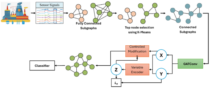
KG-EIGNN: a knowledge graph based graph neural network for fault detection in industrial systems

This paper proposes EIGNN mitigate the influence of extraneous features on fault detection. Figure 1 illustrates the two principal components of the framework: (1) an attention mechanism that transforms signals from industrial process sensors into graph data, and (2) the introduction of an instrumental variable to implement controlled manipulation by taking graphs as input, thereby providing output in EIG³³. The proposed KG-EIGNN differs from current GNN-based diagnostic models that only use structural or semantic representations. It uses exogenous intervention learning to find causal links between sensor nodes. This design helps the model separate false correlations that are caused by confounding variables, which makes it easier to understand and more reliable. KG-EIGNN also improves generalization when there is an imbalance in the data by combining supervised and contrastive learning goals. This is a problem that is often ignored in traditional hybrid models.s.

Fault detection through graph neural network

In a Graph Neural Network (GNN), sensors are represented as nodes, and the connections between them are represented as edges. This is how the defect diagnosis works. Therefore, a graph can illustrate the components of an industrial process and how they interact with one another³⁴. We can call $G=G\left(V,E\right)$ a simple graph if $V$ Is the set of all nodes and $E$ Is the set of all edges. An edge donation connects the node. $ai$ in set $R$ to edge $eib$ in set $E$. An adjacency matrix $A\epsilon\mathbb{R}N\times{N}$, where $N=\left|\text{B}\right|$, is usually used to describe the topology of a network. This means that $N$ Is the number of nodes. The letter $Aib$ stands for a link between the nodes $ai$ and $ab$. $X\epsilon{R}n\times{dn}$ shows the properties of a node, whereas $Xe\epsilon{R}c\times{dc}$ Shows the properties of an edge. GNN-based fault diagnosis aims to identify fault types.$\left\{y1\right\},\left\{y2\right\},\dots.yN\}\epsilon{Y}$ from a set of graphs $\left\{G1\right\},G2\},..GN\}\epsilon\mathcal{G}$.

An illustration of a distinctive design for graph-level defect diagnostics is presented in Fig. 2. This framework builds input graphs using three widely used techniques: KNNGraph, RadiusGraph, and PathGraph. After being processed by a GConv layer, the graphs are coarsened into subgraphs by a graph pooling layer. By lowering the input’s dimensionality, this step enhances computing performance. The node embeddings of the subgraphs are then combined into a single graph-level representation by a readout layer using operations like sum, max, and mean. Finally, a fully connected (FC) layer is used to transfer the graph representation to perform the graph-level fault diagnostics.

Graph construction with structural attribute

Based on previous work³⁵, we propose an automatic graph creation method to capture sensor interdependence in complex industrial processes. By joining segments of sensor signals that exhibit strong correlations, this technique generates a structural attribute graph. The entire graph formation process is depicted in Fig. 3.

By improving how neighboring nodes are combined, Graph Attention Networks (GAT)³⁶ allow the model to adjust the importance of each nearby node’s input. Considering a graph $G(V,E)$, the consideration coefficient of edge (i, j) is:

$${e}_{ij}=LeakyReLU\left({\varvec{a}}^{\to{T}}\left[\mathbf{W}{h}_{i}^{\to}\left|\right|\varvec{W}{h}_{j}^{\to}\right]\right),\forall\left(i,j\right)\epsilon{E}$$

(1)

Let’s ⃗ ℎ and ⃗ ℎ represent the feature vectors of nodes and , correspondingly. Matrix W is used to embed node features, while ⃗ serves as a weight vector to compute the correlation between the embedded features. To enable effective computation and comparison, the attention coefficients are normalized using the SoftMax function:

$${\alpha}_{ij}=softmax\left({e}_{ij}\right)=\frac{\text{exp}\left({e}_{ij}\right)}{{\Sigma}{k\epsilon{N}}_{i}\text{exp}\left({e}_{ik}\right)}$$

(2)

Where = { ∈ ∶ (, ) ∈ } ∪{} is the self-holding neighboring set of nodes . The new feature ⃗ ℎ′ of node can be combined by:

$${h}_{i}^{{\to}^{{\prime}}}=\sigma\left(\sum_{j\epsilon{N}_{i}}{\alpha}_{ij\varvec{W}{h}_{j}^{\to}}\right)$$

(3)

Where (⋅) is the ReLU activation function. In fault modes, where there should be substantial inter-sensor interactions represented as graph edges, the structural properties of the graph are strongly related. To record this, we sort all correlation scores. ${\alpha}_{IJ}$ And create the edge set E, from the top. $D\times{N}$ Values; the average node degree is controlled by the parameter D. Through this procedure, the structural information S can be intuitively extracted from the sensor association network $\text{G}\left(\text{V},\text{E}\right)$. As mentioned in³⁵, the apparent strength of dependence is enhanced when the attention mechanism’s receptive field is narrowed. To begin with, we use this knowledge to categorize all the industrial process’s sensors into $K=\sqrt{N}$Categories using the k-nearest neighbors (KNN) method³⁷. We use the procedure to calculate edge properties inside each set. Lastly, to finish building the whole structural attribute graph G, we repeat the technique on the K cluster centers.

GNN-based fault detection’s Graph

To understand how GNN-based fault diagnosis works in complex industrial processes, we analyze how sensor signals relate to faults. By looking at the connections between seven key elements, the cause C, the confusing factor B, the characteristics of the nodes X, the helpful factor Z, the structural details S, the graph data G, and the fault type Y, we create a Structural Causal Model (SCM)³⁸. Figure 4 shows the layout of this SCM.

$\varvec{C}\to\varvec{X}\leftarrow\varvec{B}$. The node characteristic X comes from two closely related hidden factors: the confounding variable B, which captures unnecessary sensor data, and the causal variable C, which reflects sensor signals that affect the fault mode.
$\varvec{X}\to\varvec{S}\leftarrow\varvec{Z}$. S here refers to the structural information gleaned from node properties and instrumental variables. S gathers sensor-to-sensor interactions and presents the graph structure as an adjacent matrix.
$\varvec{X}\to\varvec{Z}.$The instrumental variable Z is generated at random from the spatial properties of X.
$\varvec{X}\to\varvec{G}\varvec{{\prime}}\leftarrow\varvec{Z}$The input network is transformed into a causal graph by applying Exogenous intervention.
$\varvec{G}\to\varvec{Y}$ Making predictions about the attributes of the input graphs is the task of graph neural networks (GNNs) for fault detection. The classifier generates a prediction Y in response to the given graph G.

According to the Structural Causal Model (SCM), the total effect between $\varvec{X}$ and $\varvec{Y}$ denoted as $\text{P}\left(\text{Y}|\text{X}\right)$ differs from the causal effect of $\varvec{X}\to\varvec{Y}$,donated as (| ( = )). Causal effects account only for the direct influence of X to Y, whereas total effects include all pathways connecting X and Y. As a result, irrelevant sensor signals can act as confounding factors, introducing noise that obscures true causal relationships.

The knowledge graph was made by combining data-driven correlations from the industrial systems being studied with knowledge curated by experts. Structured consultations with domain engineers in charge of maintaining and ensuring the safety of the facilities were used to get expert knowledge. Each expert gave fault-symptom-component associations, which were checked by at least two other experts to make sure they were correct. We stored these relationships as RDF-style semantic entries in the form of triplets (component, relation, fault type). The curated knowledge was checked against historical failure logs to get rid of false or context-specific relationships. When the data was turned into a graph, the semantic relations, like “causes,” “affects,” and “co-occurs with”, were given weighted edges based on how often they appeared in the data and how sure the experts were of their accuracy. This hybrid curation process made sure that changes in fault behavior were captured while still allowing for generalization across different operational regimes.

Exogenous intervention using an instrumental variable

Any confounding variable B must be taken into account to close the gap between overall effects and causal effects. Exogenous intervention is one effective strategy³⁹. The four main categories of Exogenous interventions are instrumental variable (IV) estimates, randomized controlled trials (RCTs), back-door adjustment, and front-door adjustment. Both front-door and back-door modifications require additional observable variables. However, confounding factors are typically difficult to see in complex industrial systems, especially when the signals from faults and noises are so closely connected. Despite their effectiveness, randomized controlled trials aren’t always feasible due to their unpredictability and constant change. To get around this, we use an instrumental variable Z that allows us to eliminate false correlations without ever seeing the confounders.

The instrumental variable Z must meet three essential requirements: first, it must exhibit a strong correlation with X; second, the error terms affecting the outcome variable Y must be independent of the explanatory variable X; and third, Z must be independent of these error terms. As a result, X is the only party that can mediate the relationship between Z and Y, or, to put it another way, X is the only intermediary. According to the earlier study, we construct the instrumental variable in two steps⁴⁰. First, we regress X on Z to estimate the coefficient , which is equal to $\mathbf{C}\mathbf{o}\mathbf{v}(\mathbf{X},\mathbf{Z}).$Next, we substitute the expression for Z with one that includes Y, and then perform a regression of Y on Z denoted as $\mathbf{C}\mathbf{o}\mathbf{v}(\mathbf{Y},\mathbf{Z}).$ When comparing Y and Z, the definitional limitations of Z lead to bias in the results.

$$\text{X}={\upalpha}\text{Z}+{\upepsilon}\text{X};\text{Y}={\upomega}\text{X}+\text{{\rm\:E}}\text{y}$$

(4)

Here and are error terms that include confounding variable B. After these adjustments, the estimated effect of X on Y becomes asymptotically unbiased.

$$\omega=\frac{\frac{1}{n}\sum_{i=1}^{n}\left({z}_{i}-\stackrel{-}{z}\right)\left({y}_{i}-\stackrel{-}{y}\right)}{\frac{1}{n}{\sum}_{i=1}^{n}\left({z}_{i}-\stackrel{-}{z}\right)\left({x}_{i}-\stackrel{-}{x}\right)}=\frac{Cov\left(Z,Y\right)}{Cov\left(Z,X\right)}$$

(5)

Exogenous intervention learning

Instrumental variable generation

For instrumental variables to be deemed limited, they must meet two primary criteria: first, Z must have a causal effect on the covariates X and only influence the prediction through its effect on X. By these rules, we use random perturbations as an independent variable, drawing inspiration from previous data augmentation attempts⁴¹. More specifically, we randomly perturb the node properties X to create Z. This method meets the basic needs of instrumental variables because (6) random changes do not directly influence the prediction results and (7) they alter the features and layout of nodes in the graph, which indirectly impacts the prediction. The first step in developing an instrumental variable is to establish a $\varvec{Z}\to\varvec{X}$ Causal link. After aligning the one-hot label Y with X using a graph attention layer, we concatenate the two to produce an updated representation of X. The representation of X is enhanced by this process. The instrumental variable Z is created from the combined X and Y using an encoder made up of two graph attention layers and multilayer perception (MLPs). The MLP is used to determine the mean and standard deviation of the latent space corresponding to the intervention variables.

$${X}_{att}=GAT\left(X,Y\right)$$

(6)

$$\mu,\sigma=encoder\left({X}_{att},Y\right)$$

(7)

Instrumental variable Z is a random matrix that obeys a normal distribution with mean and standard deviation .

Exogenous intervention

A and C are each spliced after one layer of the graph attention network to obtain the reconstruction. ${A}_{recon}$.

$${C}_{att}GAT\left(C,B\right)$$

(8)

$${A}_{recon}=GAT\left({A}_{att},{C}_{att}\right)$$

(9)

$${A}_{recon}=\sigma\left(f\left({A}_{recon}\right)\right)$$

(10)

where (⋅) is the sigmoid activation function and (⋅) is a liner layer. We select the binary cross-entropy (BCE) function to compute the reconstruction loss:

$${\mathcal{L}}_{R}={f}_{YZV}\left(A,{A}_{recon}\right)$$

(11)

The GNN-based fault diagnosis is a classification task, as detailed in Sect. 1. Given a set of graphs $\{\text{G}1,\text{G}2,\dots,\text{G}\text{N}\}\in\mathfrak{H}\mathfrak{}$ With fault types, we use the negative log-likelihood (NLL) function to compute the classification loss.

$${\mathcal{L}}_{Z}=-\sum_{i=1}^{N}\sum_{j=1}^{M}{Y}_{j}\text{log}{q}_{j}\left(\mathcal{W}|{G}_{i}\right)$$

(12)

Here is used as the hyper-parameters of the model, the ground-truth label is described as , and denotes the probability of related to the fault type .

It is important to note that the model cannot entirely disregard the raw data, as doing so would conflict with conventional fault detection process. To achieve symmetry and combine the reconstruction loss, we established the tuning parameters 1 and 2. There are three types of loss in this model one are the ${\mathcal{L}}_{R}$, second is Exogenous intervention loss ${\mathcal{L}}_{IV}$, and the third one is fault diagnosis loss ${\mathcal{L}}_{C}$. The total loss of the model KG-EIGNN is represented as ${\mathcal{L}}_{TOTAL}$, and the comprehensive implementation of KG-EIGNN in Algorithm 1.

$${\mathcal{L}}_{TOTAL}={\mathcal{L}}_{Z}+{\lambda}_{1}{\mathcal{L}}_{IV}+{\lambda}_{2}{\mathcal{L}}_{R}$$

(13)

For a specific stochastic perturbation , we have ${z}_{i}=\text{f}(\text{x},{z}_{i})\approx{{\upalpha}}_{i}\cdot\text{x}.{\upalpha}$Is a self-learning parameter, which is used to represent the relationship between and . Substituting the relation above between the original feature and the augmentation feature ${x}_{{z}_{i}}$ Into Eq. (13), we will get the ${y|}_{x={z}_{i}}$ With different proportionality coefficients .

$${y|}_{x={z}_{i}}={W}_{xy}\cdot{z}_{i}+{W}_{cy}\cdot{c}+{\widehat{\mathcal{E}}}_{y}={\alpha}_{i}\cdot{W}_{xy}\cdot{x}+{W}_{cy}\cdot{c}+{\widehat{\mathcal{E}}}_{y}$$

$$={\alpha}_{i}{y\mid}_{do\left(x=x\right)}+{W}_{cy}\cdot{c}+{\widehat{\mathcal{E}}}_{y}$$

(14)

Where ${y|}_{do\left(x=x\right)}$denotes causal path $X\to{Y}$. Substituting the ${y|}_{x={z}_{i}}$ With Eq. (14) obtained by learning, we get the learning object from the instrumental variable estimation. The advantage is clearly that we can suppress the confounding effect without straight perceiving the confusing variable B. The objectives of Exogenous intervention learning can be concluded as:

$${\mathcal{L}}_{IV}=min\sum_{i\ne{j}}\left({\alpha}_{i}-{\alpha}_{j}\right)\cdot\left({W}_{by}\cdot{b}+{\widehat{\mathcal{E}}}_{y}\right)$$

(15)

Source link