Ethics statement
The use of human genetic data in this study was approved by the University of California, San Diego, Institutional Review Board.
Genome-wide association and genotype imputation
For the MHC analysis, we compiled genotype data from 10,107 T1D and 19,639 nondiabetic individuals of European ancestry across five cohorts (Supplementary Table 1). Cohorts were selected based on the availability of genome-wide genotyping array data for imputation into the TOPMed r3 panel24,37,38 and the MHC locus using the Michigan HLA reference panel39 and several cohorts (GENIE ROI, CSGNM) were further excluded due to lower quality imputation at this locus. T1D cases were matched to nondiabetic individuals by ancestry and, where possible, genotype array9. We performed quality control on variants using the HRC imputation preparation program (v4.2.9, https://www.well.ox.ac.uk/~wrayner/tools/) and PLINK (v1.9)to remove variants with MAF < 1%, missing genotypes >5%, violating Hardy-Weinberg equilibrium (HWE, P < 1 × 10⁻⁵ in unaffected cohorts; HWE, P < 1 × 10⁻¹⁰ in case cohorts), allele ambiguity and difference in allele frequency >0.2 compared to HRC r1.1 reference panel38,40. We imputed 55,615 variants from the four-digit multi-ethnic HLA reference panel (v1). We retained variants with imputation accuracy (r2) > 0.5 and a standard deviation in nondiabetic allele frequency < 0.055 for association testing41.
To examine genetic risk outside the MHC, we compiled association data from 20,355 T1D cases and 797,363 nondiabetic European ancestry individuals, matched by ancestry and genotype array where possible (Supplementary Table 11). For the FinnGen cohort, we downloaded the summary statistics from the r10 version of ‘T1D_Early’, which includes 2,832 individuals diagnosed with T1D under the age of 20 years and excludes individuals with T2D.
We used genotyping data for 263 individuals from nPOD, including 115 T1D cases and 148 individuals without T1D42. Additionally, we used 1,999 T2D individuals from the WTCCC1 cohort43. To examine the predictive ability of T1GRS in individuals of African ancestry, we used 284 T1D individuals from SEARCH and 404 nondisease individuals from CLEAR44,45. For all cohorts, we performed variant quality control as described above before imputation using the Michigan HLA and TOPMed r3 panels.
We considered participants with whole-genome sequencing and EHR data from the AoURP Controlled Tier Dataset v7 (ref. 46). T1D and nondiabetic individuals were identified using a combination of diagnosis codes (ICD-9/ICD-10) and drug exposures extracted from the EHR data. Briefly, a participant was classified as having T1D if they met all of the following criteria: (1) an ICD-9/ICD-10 diagnosis code for T1D on at least three visits or self-reported T1D on enrollment survey; (2) three or more instances of a recorded insulin prescription; (3) did not have a diagnosis of cystic fibrosis, secondary diabetes mellitus and drug- or chemical-induced diabetes mellitus; and (4) were not prescribed any other oral or injectable hypoglycemic agents. A participant was identified as nondiabetic if they did not have any of the following: (1) an ICD-9/ICD-10 code corresponding to T1D/T2D or self-reported T1D, or (2) an insulin prescription. Diagnosis codes used for classification were as follows: T1D—ICD-9-CM 250.x1, 250.x3; ICD-10-CM E10.x; T2D—ICD-9-CM 250.x0, 250.x2; ICD-10-CM E11.x; cystic fibrosis—ICD-9-CM 277.00–277.09; ICD-10-CM E84.x; secondary diabetes mellitus—ICD-9-CM 249.x and ICD-10-CM E08.x, E13.x; and drug-induced or chemical-induced diabetes mellitus—ICD-10-CM E09.x.
For insulin drug exposures, we included all medications classified under the ATC code A10A, including fast, intermediate, long, combination and inhaled insulins. Noninsulin hypoglycemic agents were defined by ATC code A10B and include biguanides, sulfonylureas, α-glucosidase inhibitors, thiazolidinediones, dipeptidyl-4 inhibitors, glucagon-like peptide 1 analogs, sodium-glucose cotransporter 2 inhibitors, meglitinides and their combinations.
Complications were defined by the presence of an ICD-9/ICD-10 code related to the complication. Cardiovascular complications were defined as myocardial infarction, cerebral infarction, heart failure, major vessel atherosclerosis, renal disease identified as a diagnostic code of diabetes and any severity of renal disease or separate ICD-9/ICD-10 code of proteinuria. Neuropathy was defined as any diagnostic code listing diabetes and any severity of neurologic complication. Retinopathy was defined using the following codes: cardiovascular—ICD-9-CM 410.7, 410.1x, 410.4x, 410.6x, 410.9x, 410.9, 428.xx, 434.x1, 437.0, 440.0, 440.1, 440.8; ICD-10-CM 121.x, 150.x, 163.x, 167.2, 170.0, 170.1, 170.8; nephropathy—ICD-9-CM 249.4x, 250.4x, 791.0; ICD-10-CM E08.2x, E09.2x, E10.2x, E11.2x, E13.2x, R80.x, N06.x; neuropathy—ICD-9-CM 250.6x, 249.6x; ICD-10-CM E08.4x, E09.4x, E10.4x, E11.4x, E13.4x; and retinopathy—ICD-9-CM 362.0x and 250.5x; ICD-10-CM E08.3x, E09.3x, E10.3x, E11.3x, E13.3x.
Details of the generation and quality control of the genomic data are provided in the AoURP Genomic Quality Report, release C2022Q4R9. Briefly, we used computed genetic ancestries provided by AoU to identify participants of European Ancestry. Genomic quality control and imputation were performed as described above for research participants.
Association testing and meta-analysis
We used the first bias-corrected LogReg in EPACTS (v3.3.0, https://genome.sph.umich.edu/wiki/EPACTS) and variants for association with MAF > 1% at the MHC locus and MAF > 0.1% genome-wide were tested, including the first four genotype PCs and sex as covariates. In the MHC locus, we tested variants for association across a 4 Mb locus on chromosome 6 spanning 30–34 Mb (hg19). For both MHC-specific and genome-wide association analyses, we combined summary statistics from all tested cohorts using a fixed-effects inverse variance-weighted meta-analysis. For new loci, we considered variants with P < 1 × 10⁻⁸, identified as a more appropriate significance threshold for MAF > 0.1% variants47. For replication analyses, we updated the meta-analysis by replacing the summary statistics for the ‘T1D_EARLY’ phenotype in Finngen with those from the more recent r12 version, which includes an additional 219 T1D cases and 409,349 nondiabetic individuals. From the meta-analysis, we estimated the degree of confounding using LD score regression48 by calculating the intercept from one (0.0844), which supported a minimal effect of residual population structure on the results.
Conditional analysis of independent signals
To identify independent signals at the MHC locus, we performed stepwise conditional analyses by including the most significant variant from each meta-analysis as a covariate in the association tests for each cohort, followed by reperforming through meta-analysis. We repeated this process by iteratively adding each new variant to the model until no variants remained significant at P < 5 × 10⁻⁸, where this threshold was selected based on testing variants with MAF > 1%. We also performed a ‘preconditional’ analysis to examine the effect of signals outside of 70 established class I and II HLA risk alleles and 20 DR3/DR4 pairwise HLA haplotypic and allelic interactions24,49,50,51. We added 90 covariates into the model to capture the additive effect of each alternate allele across 70 HLA risk alleles, and a binary column for each of the 20 interactions, before performing association testing and meta-analysis. We then performed stepwise conditional analyses by iteratively adding the most significant variant as an additional covariate in the model and reperforming the meta-analysis until no variants remained significant at P < 5 × 10⁻⁸.
Credible set generation for signals in the MHC
For all independent signals identified at the MHC locus through stepwise conditional analysis, we generated 95% credible sets. We first identified variants in linkage with the lead variant for each signal (r2 > 0.1) and we calculated the Bayes Factor for each variant based on the effect and standard error as described by Wakefield52. We generated PIP scores by dividing the Bayes Factor by the total sum of the Bayes Factors for all variants in the set. We included variants up to the 95% threshold in each credible set.
SuSiE fine-mapping of the non-MHC loci
We used SuSiE (v0.11.42) to fine-map loci identified through two rounds of variant clumping using PLINK (v1.9; ‘–clump-p1 5e-8 –clump-p2 0.05 –clump-r2 0.1 –clump-kb 10000’; ‘–clump-p1 5e-8 –clump-r2 0 –clump-kb 500’). We generated loci 500 kb around the variants in each clumped region, considering all variants regardless of MAF. We identified 87 significant loci and included 10 additional known loci not reaching genome-wide significance (CDKN1C, CYP27B1, LMO7, CCR7, 17q24, ACOXL, CCR5, IRF2, TAGAP, 6q27) for a total of 97 loci. We created 95% credible sets for each locus in SuSiE using genotypes from six dbGAP cohorts, including 32,518 individuals (DCCT, GENIE ROI, GENIE UK, GoKIND, T1DGC and WTCCC1) to define the LD matrix and set parameters to ‘L = 10, coverage = 0.95, min_abs_corr = 0.01, max_iter = 50,000’. For complex loci with multiple signals identified in a previous study (DLK1, IFIH1, TYK2, IL10, PTPN2, AIRE, UBASH3A, CTLA4, IL2RA), we recomputed the meta-analysis using only the six dbGAP cohorts with genotype data included in the LD matrix above9. Lead variants were defined as the variant with the largest PIP for the signal. We defined new loci as variants that reached genome-wide significance and mapped > 500 kb from other known loci.
Annotations of credible sets
We leveraged genomic datasets to examine preferential TF binding to annotate new credible sets. We overlapped all credible set variants with accessible chromatin peaks in 46 immune and 12 pancreatic cell types26,53. We tested each variant for preferential allelic binding to TF motifs using FIMO (v4.12.0)54. We also leveraged databases such as GTEx and JASPAR to annotate credible set variants55,56.
Constructing a nonlinear machine learning polygenic risk score
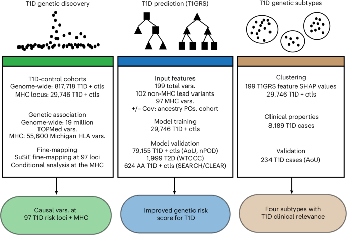
We leveraged 199 variants, including the lead variants from 27 MHC signals, 70 established HLA-associated alleles and 102 non-MHC lead variants (including five putative loci). We developed two models based on the CatBoost classifier framework (v1.0.6), one with the 199 variants alone (‘T1GRS-var’ model) and another with additional covariates of sex, PC1-4 and binary covariates for each cohort (‘T1GRS-cov’ model). This approach generates a probability ranging from 0 to 1 that represents the model’s confidence that an individual has T1D, which can be treated as a GRS. We refer to this probability as a ‘score’ to avoid confusion that it represents the actual probability of T1D. The discovery dataset, comprising five cohorts with 10,107 T1D and 19,639 unaffected individuals, was combined into a single genotype matrix, which was randomly split into ten subsections for cross-fold validation. Across ten iterations, a model was trained on 90% of the data and evaluated on the remaining 10% (as outlined previously57). Hyperparameters were determined by exhaustive grid search on the first cross-validation fold of the discovery dataset. Briefly, we used a binary CatBoostClassifier with 254 estimators, a depth of 5, a learning rate of 0.12 and a gradient boosting method. Specific hyperparameter settings are available at https://github.com/Gaulton-Lab/t1d-grs-analysis-catboost.
The probability scores for individuals in each testing fold were recorded and used to calculate the overall AUC of the model. This process was identical in the T1GRS-cov and T1GRS-var models, including all variant, MHC-only and non-MHC submodels. A representative model for each evaluation was trained on all individuals for validation purposes. Independent validation was performed on the NIH AoU Research Cohort containing 234 T1D and 78,658 nondiabetic individuals and the nPOD cohort, comprising 115 T1D and 148 nondiabetic individuals. A standard random seed was set to ensure reproducibility and a frozen model with identical hyperparameters was used for every validation.
Generation of a LogReg comparison model
As a comparison to our T1GRS model, we also built a LogReg classifier. This model learns a single weight for each feature and performs a linear combination to predict the probability of T1D. The model outputs a probability score between 0 and 1. To prevent overfitting and allow the model to learn weaker non-MHC-based predictors of T1D, we applied strong L2 regularization (C = 0.001). The LogReg model was trained and evaluated using the same tenfold cross-validation format as all T1GRS models, using the same seed and training data.
Feature importance and interaction analysis
Feature importance and interaction within nonlinear models were calculated using the SHAP machine learning interpretability suite (v0.41.0)58. SHAP is an approach to explain the output of any machine learning model based on cooperative game theory and the concept of Shapley values. SHAP values assign each feature an importance value for a particular prediction in the context of a specific model. The magnitude of feature importance is determined by the mean absolute value of all SHAP values for a given feature. SHAP values also capture nonlinear interactions between features on a per-individual basis and enable ranking pairwise feature interactions by magnitude. Each model was run through the standard SHAP pipeline and feature importance was recorded. Feature interaction analysis was performed using the shap_interaction_values function. To identify significant feature interactions, we converted all pairwise interaction values to z scores and calculated P values for each interaction using a z test. We then applied FDR correction to P values.
Complexity scores
To understand how complex a model’s decision is for an individual’s disease classification, we developed a ‘complexity’ score, which is the total displacement of SHAP values for an individual, calculated by summing the absolute values of each feature, resulting in a single score per individual. A lower complexity score suggests a more straightforward classification, for example, driven by one or a few highly influential factors. For example, an individual with a strong MHC signal as the primary driver for a positive classification and minimal influence from other non-MHC features would likely exhibit a low score. Conversely, a higher complexity score indicates that many features, each contributing a smaller amount, collectively lead to the disease outcome. Individuals were assigned to deciles based on their complexity scores.
Defining genetic subtypes and validation
Individual-specific SHAP feature contribution vectors from the T1GRS-var model formed the basis of this analysis for both discovery and validation cohorts. All analyses were made reproducible by using a fixed random seed. Starting with the discovery cohort, high-dimensional SHAP vectors were first reduced using PCA, retaining up to 175 principal components. We then employed high-dimensional clustering in ScanPy (v1.8.2)59 as follows: in PCA space, a k-nearest neighbor graph was constructed (using 120 neighbors). This graph was then used to generate a two-dimensional UMAP embedding, with a ‘min_dist’ parameter of 0.25. Subgroups of individuals within the discovery cohort were then identified by applying the Leiden community detection algorithm to the kNN graph, using a resolution of 0.05. Next, we used the ScanPy ingest workflow to project the validation cohort onto our existing clusters. To assign validation individuals to the clusters, PCA representations were projected into the discovery cohort’s UMAP space and then assigned to clusters using the same Leiden algorithm.
Analysis of age of onset, clinical complications and T2D loci in T1D subtypes
To identify differences in age of onset between clusters, we performed a log-rank test and considered significant differences at P < 0.05. To identify differences in clinical complications between clusters, the OR was calculated in the discovery and AoU datasets and P values were calculated using a Cox proportional hazards test. To determine enrichment of T2D loci within clusters, we defined T1GRS variants in LD (r2 > 0.2) with reported T2D variants60. We performed LogReg for each cluster using mean-normalized SHAP values for each locus as the predictor and T2D association as the binary outcome.
Analysis of T1D GRS
We calculated GRS2 using 60 exact TOPMed variants, 2 exact Michigan HLA for rs116522341, rs1281934, and the proxy variants DQB1*06:02, B*18:01, DPB1*03:01, rs1611547 and rs114170382 from Michigan HLA for rs17843689, rs371250843, rs559242105, rs144530872 and rs149663102, respectively. In GRS2, we excluded individuals with more than two HLA-DR/DQ proxy SNPs according to the published methods16. Within each GRS, we examined the total GRS and its components of MHC and non-MHC variants. We calculated the AUC for the receiver operating characteristic analysis to assess the differentiation power of each GRS for T1D. We then tested the differences between AUCs using the DeLong test. First, we compared T1GRS and GRS2 in individuals with T1D and those without using both the ‘T1GRS-cov’ and the ‘T1GRS-var’ models. Next, we validated T1GRS using individuals in the nPOD biorepository to differentiate between T1D and nondiabetes and using the T1D from nPOD and 1,999 T2D from WTCCC1 (ref. 43).
We calculated a published African ancestry risk score in 284 T1D and 404 nondiabetic individuals from SEARCH and CLEAR to compare with T1GRS44,45. We used TOPMed to impute rs34850435, rs9271594, rs9273363, rs2290400 and rs689, while Michigan HLA was used to impute rs2187668. The variant rs9268838 was used as a proxy for rs34303755 (r2 = 0.849, D′ = 1.0 in African ancestry).
Lastly, we generated a scale for T1GRS scores using the number of individuals with T1D at various percentiles and calculated a diagnostic for each GRS value using the Youden index (sensitivity + specificity − 1). We calculated sensitivity at each GRS score on the scale as TP/(TP + FN) and specificity as TN/(TN + FP)61. We defined DR3/DR4 individuals using four-digit HLA alleles imputed from the T1DGC reference panel using SNP2HLA32. DR3 status was classified as HLA-DRB1*03:01–DQB1*02:01, while DR4 as HLA-DRB1*04:01/02/04/05/08–DQB1*03:02/04/02:02 (ref. 33).
Variant category classification
To assign variants used in T1GRS to cell types, we first intersected credible sets with the cell-type atlas of cis-regulatory elements (CATlas)53 for pancreatic and immune cell types. For loci that did not intersect these cis-regulatory elements, we determined credible set intersection with gene bodies in GENCODE GRCh38.p14 (ref. 62) and annotated loci with cell types based on gene expression patterns. Lastly, for several loci previously linked to specific genes, we annotated loci to cell types based on the expression patterns of these genes. The full list of links between loci in T1GRS and cell types, as well as the references for the links, is provided in Supplementary Table 18.
Intersection of cluster loci and cell-type regulatory elements
To identify the top loci for each cluster, SHAP values were averaged across all individuals within the cluster. For each T1GRS variant, SHAP values were normalized across clusters to sum to 1. We identified loci for each cluster with a normalized SHAP value greater than 0.75. Using the top loci for each cluster, credible sets for these loci were intersected with regulatory elements for 12 immune and pancreatic endocrine cell types derived from ENCODE. For each cluster, the posterior probability of association for all variants intersecting a regulatory element in a cell type was summed. Permutation testing was performed by shuffling the cumulative probability of associations across all cell types 10,000 times for each cluster and calculating a P value from this null distribution.
Reporting summary
Further information on research design is available in the Nature Portfolio Reporting Summary linked to this article.


