Optimal invariant sets for atomistic machine learning

Overall strategies

The aim of this work is to apply strategies of optimal pattern recognition to problems for atomistic machine learning. We will begin in the “Pattern recognition based on the method of Langbein and flexible descriptor sets” section by explaining these strategies in the abstract, applied to a generic set of invariant features, to assemble reduced sets of invariant features. These reduced sets are independent in a nonlinear sense, using a local test. We also explain the need for constructing flexible sets that are functionally independent in a global sense. In “The ACE basis” section, we review how spherical tensors are used to build potentials in linear ACE, and in “A functionally-independent subset for ACE” section, we then explain how to apply the aforementioned filtering strategies to reduce the basis set of the ACE, which uses these spherical tensors. In the “Cartesian formulation of tensors and enumeration of invariants as graphs” section, we review an alternative to the spherical strategy for enumerating a set of invariants, instead using the equivalent Cartesian tensor formulation. Using Cartesian tensors, the simple invariant expressions correspond to multigraphs. Passing these multigraphs through the flexible-basis search methods yields a relatively small set of tensors that extracts all functionally independent information from a function on the sphere. This set does not grow combinatorially in the expansion order, instead growing only quadratically, which is asymptotically identical to the number of degrees of freedom in the tensors themselves⁵⁴. Finally, in the “Incorporating flexible bases into atomistic neural networks” section, we detail how we have incorporated this set of invariants into a neural network architecture based on HIP-NN, which we call HIP-HOP-NN.

Pattern recognition based on the method of Langbein and flexible descriptor sets

Moment invariants⁶⁵, which themselves have been used for MLIPs^16,66, have been studied extensively in the field of pattern recognition. 3D geometric moments are projections of a scalar function $f:\,{{\mathbb{R}}}^{3}\to {\mathbb{R}}$ to the monomial basis. The moments of each order ℓ form a moment tensor

$${\scriptstyle{\ell}\atop}{M}_{{\alpha }_{0}…{\alpha }_{l-1}}=\int \,{r}_{{\alpha }_{0}}…{r}_{{\alpha }_{\ell -1}}f({\bf{r}}){d}^{3}{\bf{r}}$$

(1)

of rank ℓ⁶⁷, where the α_i ∈ {1, 2, 3} indicate one coordinate of ${\bf{r}}\in {{\mathbb{R}}}^{3}$. Products and contractions of tensors are tensors, and zeroth-rank tensors are invariant to rotations. This allows us to generate sets of invariant descriptors by multiplying and contracting moment tensors in all combinations. A key drawback is that this produces a vast number of invariants, and most are redundant in some way.

Optimal bases of moment invariants in pattern recognition are complete, functionally independent, and flexible⁵³. Complete means that any two functions that differ by more than a rotation have different descriptors. Functionally independent means that no descriptor can be written as a function of the others. Flexible means that the basis never becomes degenerate. These three criteria guarantee that the basis has the ability to distinguish any variation in the configurations and the smallest possible size.

The set of all possible total contractions of the moment tensors forms a complete set of rotationally invariant descriptors, but the size of this set scales combinatorially with the maximum tensor order. The number of functionally independent moment invariants is given by the number of moments minus the dimensionality associated with the symmetry operation, which is, in this case, the three parameters required to specify a rotation. A functionally independent set can theoretically be identified using the Jacobi criterion⁵². The key is to recognize that if an invariant I_n(m) as a function of the underlying moments m is functionally dependent on other I₀(m), …, I_n−1(m) invariants, then we can write an implicit function f for I_n(m):

$${I}_{n}(m)=f({I}_{1}(m),\ldots ,{I}_{n-1}(m)).$$

(2)

As a consequence, the derivatives of the moments must be linearly dependent on each other, as

$$\frac{\partial {I}_{n}}{\partial m}=\mathop{\sum }\limits_{i=1}^{n-1}\frac{\partial f}{\partial {I}_{i}}\frac{\partial {I}_{i}}{\partial m}$$

(3)

implies that the Jacobian of the moments, $\frac{\partial {I}_{i}}{\partial m}$, does not have full rank. By testing the Jacobian on candidate sets of moments, one can assemble a set of moments that is complete up to symmetry. Instead of analytically solving for the rank of the Jacobian, Langbein and Hagen developed an approximation algorithm that randomly assigns values to the moments and solves for the rank numerically⁴⁹.

Combinatorially scaling sets of functionally dependent tensor contractions has also been used in atomistic machine learning as Moment Tensor Potentials (MTP)¹⁶. The moment tensors have the attractive property of extracting linearly independent features from an atomic environment in a systematic way and forming a complete basis for regression.

One of our contributions is recognizing that the strategy of Langbein and Hagen is applicable to filtering down any set of invariants used for featurizing a symmetric space, and in particular for atomic environments. The use of moment invariant methods from the 3D imaging community has been previously studied⁶⁶, but in our work we show that the approach of Langbein and Hagen can be applied to a far wider range of descriptors than moment invariants alone, yielding more expressive ML models and improved results, and identified the necessity to invoke additional learning machinery, such as a neural network, over the moment invariants.

Bujack et al. realized that the Langbein approach would not necessarily work when applied to certain patterns⁵¹. This is because when symmetry causes a moment to vanish, a large number of moment invariants will vanish with it. As such, a set of invariants can be complete in a local region, but incomplete when considering the entire space of patterns. This necessitates building a flexible basis: one that is complete across the space of possible patterns to detect. This issue becomes particularly important for applications in atomistic machine learning because the spherical nature of the functions causes naive bases of moment invariants to degenerate to incompleteness as discussed in ref. ⁵⁴. In this paper, we focus on demonstrating the applicability and effectiveness of this technique and not on the theoretical foundations. Explicit examples and the full derivation of a flexible set from irreducible tensors are given in the companion paper⁵⁴.

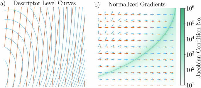
The situation is depicted schematically in Fig. 1. A set of descriptors is used to identify points on a manifold, in this case, the underlying plane. The x and y axes are two moments, and the values of the functions as shown through iso-contours are two moment invariants. Locally at each point, the rank of the Jacobian of the descriptors corresponds to the dimension of the space spanned by the gradients of the descriptors at that point. Across most of the plane, these descriptors are functionally independent; the gradients are not parallel, so the rank of the Jacobian is two, and the Langbein algorithm identifies the descriptors as containing functionally independent information. However, there is a sub-manifold on which these descriptors are actually functionally dependent on each other: on this sub-manifold, the level curves are parallel, the gradients are parallel, and the condition number of the Jacobian diverges because its rank is one. In other words, there is a line of critical points. Note that this does not require that the descriptors be linearly dependent on this manifold. As such, these two descriptors do not provide a flexible set for characterizing the plane. One can also see this by tracking the intersection of the descriptors: for the level curves that intersect with the degenerate manifold, the descriptor level curves intersect at two points, and there is a set of points on one side of the degenerate manifold whose descriptors are identical to those found on the other side of the manifold. This means that the values of the descriptors are identical at these two locations even though the values of the coordinates are different, illustrating that non-flexible bases can fail to differentiate even where they are not degenerate.

The ACE basis

Here, we briefly review the ACE basis for constructing features using spherical tensors. For a pedagogical discussion of spherical tensors for representing atomic environments, see Supplementary Note 1. We use the notation of ref. ³⁴ limited to one element type. The atomic basis is defined as

$${\alpha }_{nlm}=\mathop{\sum }\limits_{\begin{array}{c}j\end{array}}{\phi }_{nlm}({{\bf{r}}}_{ji})$$

(4)

$${\phi }_{nlm}({\bf{r}})={R}_{nl}(r){Y}_{l}^{m}(\widehat{{\bf{r}}}),$$

(5)

where R_nl is a radial basis function and ${Y}_{l}^{m}$ is a spherical harmonic function^34,36. Because of the large number of indices associated with the atomic basis, they are collected into a single product-index v = (n, l, m) in future formulas. A permutation-invariant basis function is constructed by forming products of the atomic basis:

$${A}_{{\bf{v}}}=\mathop{\prod }\limits_{t=1}^{\omega }{\alpha }_{{v}_{t}},\,{\bf{v}}=({v}_{1},\ldots ,{v}_{\omega }).$$

(6)

Rotational invariance is then achieved by the following formula, constituting an average of the multi-particle basis over all possible rotations:

$${B}_{{\bf{v}}}={\int }_{\hat{R}\in O(3)}\mathop{\prod }\limits_{t=1}^{\omega }{A}_{{v}_{t}}(\{\hat{R}{{\bf{r}}}_{ij}\})\,d\hat{R}$$

(7)

$$=\mathop{\sum }\limits_{{{\bf{v}}}^{{\prime} }}{C}_{{\bf{v}}{{\bf{v}}}^{{\prime} }}{A}_{{{\bf{v}}}^{{\prime} }},$$

(8)

where the coefficients ${C}_{{\bf{v}}{{\bf{v}}}^{{\prime} }}$ are sets of combined Clebsch-Gordan coupling coefficients that compute a scalar component of each element of v. The matrix of Clebsch-Gordan coupling coefficients is extremely sparse; many elements of ${A}_{{\bf{v}}}^{{\prime} }$ are rotationally covariant and so they average to zero; these elements are ignored for computational purposes. In a linear ACE model, the energy at site i is then given by

$${E}_{i}=\sum {c}_{{\bf{v}}}{B}_{{\bf{v}}}={\bf{c}}\cdot {\bf{B}}.$$

(9)

A relevant aspect of ACE is that the basis A_v, being formed of products, grows exponentially in ω, which controls the maximum body-order of the features. This combinatorial growth propagates to the number of invariant features B; for practical purposes, one needs to define limitations on the maximum n, l, ω.

For the computational studies in this work using ACE, the ACEpotentials.jl code described in ref. ⁵⁶ was used. The linear solver used for the Langbein algorithm is the rank-revealing QR factorization (RRQR) algorithm. This solver was chosen as it allows for fitting to singular matrices that occur at higher degrees. The performance of the RRQR solver compared to the QR solver was verified for Ni across polynomial degrees, and the difference in test set error for the solvers was less than 10⁻⁹. In this work, the weighting parameter between the radial and spherical harmonic components was set to 1.0, and the order was set to four.

A functionally independent subset for ACE

The combinatorially scaling number of features in ACE is not inherent to the problem but a result of many of the features containing redundant information in the form of functionally dependent descriptors. For regression problems, this redundant information can be useful for producing more expressive regression models. In this work, we adapt Langbein’s algorithm to construct a functionally independent subset of the ACE basis. This means that while maintaining ACE’s ability to distinguish any variation in the configurations, we remove all descriptors that are functions of others to produce the smallest possible set that satisfies completeness. A similar approach is used in ref. ⁶⁶ but applied to Zernike moments rather than ACE descriptors. Our computation includes the following stages:

Construct a matrix of $\frac{\partial {B}_{{\bf{v}}}}{\partial {\alpha }_{j}}$ for one atom (from random neighbors). The α_j term is the atomic basis used to form B_v through sums and products. The components $\frac{\partial {B}_{{\bf{v}}}}{\partial {\alpha }_{j}}$ are calculated numerically.
Initialize a candidate Jacobian matrix with columns equal to the number of atomic basis functions (α_v) and initially empty of rows.
For each B_v until the utmost number of B_v terms is reached: compute whether appending the row vector of partial derivatives of the invariant will augment the rank of the candidate Jacobian matrix. If the rank is increased, append the partial derivatives of the invariant to the candidate Jacobian matrix. From this, construct an index of B_v components that increase the rank of the candidate Jacobian matrix.
Repeat this N times (where N is the number of data points sampled). Each repetition produces a new set of indices. A B_v member only needs to be identified as increasing the candidate Jacobian matrix rank for one data point to be included in the final subset.

Using this algorithm, a subset of basis functions is selected. For one data point, the maximum number of basis functions B_v selected is equal to the size of the set α—as the largest possible rank is the minimum dimension of the matrix. However, with multiple data points sampled, the size of the final functionally independent subset can be larger than the size of the set α. This is because different numerical values can select varying subsets of B_v.

In the Langbein algorithm, a numerical value is used to compute the $\frac{\partial {B}_{{\bf{v}}}}{\partial {\alpha }_{j}}$ matrix at a set point. This number can be generated from a random distribution (a random data point), or it can be selected from the training data. The difference in the Langbein algorithm’s performance with random data points and training data was investigated in preliminary work. Random data points more effectively sample the space of possible values, and were subsequently used in the algorithm as default. This also means that the subset of points chosen by the Langbein algorithm is independent of the training set used. Supplementary Fig. 2 illustrates the preliminary work performed.

Cartesian formulation of tensors and enumeration of invariants as graphs

In the companion paper, the authors generate a flexible set by computing the Cartesian moment tensors (1) as projections of the functions to the monomial basis and deriving their irreducible tensor decomposition by subtracting their traces⁵⁴. The irreducible tensors${T}_{\overrightarrow{{\boldsymbol{\alpha }}}}^{\ell }({\bf{r}})$⁶⁸ are the traceless fully symmetric tensors. They are the Cartesian equivalent of the spherical harmonics. They form the building blocks of the flexible set and are multiplied and contracted to form invariants. In this paper, we deal with spherical functions only. In contrast to general volumetric functions, the traces of the moment tensors are linear multiples of lower-rank moment tensors and do not need to be considered. The irreducible decomposition simplifies to a single full-rank irreducible tensor. Therefore, instead of removing the trace of moments in the monomial basis, we can directly compute the irreducible moment tensor by projecting the function onto the traceless part of the monomial tensors r^⊗ℓ. The first three irreducible tensors ${T}_{\overrightarrow{{\boldsymbol{\alpha }}}}^{\ell }({\bf{r}})$, where $\overrightarrow{\alpha }=({\alpha }_{1},{\alpha }_{2},…{\alpha }_{\ell })$ take the shapes

$$\begin{array}{lcl}{T}^{0}({\bf{r}}) & = & 1\\ {T}_{{\alpha }_{0}}^{1}({\bf{r}}) & = & {r}_{{\alpha }_{0}}\\ {T}_{{\alpha }_{0}{\alpha }_{1}}^{2}({\bf{r}}) & = & {r}_{{\alpha }_{0}}{r}_{{\alpha }_{1}}-\frac{1}{3}{\delta }_{{\alpha }_{0}{\alpha }_{1}}{r}^{2}\\ {T}_{{\alpha }_{0}{\alpha }_{1}{\alpha }_{2}}^{3}({\bf{r}}) & = & {r}_{{\alpha }_{0}}{r}_{{\alpha }_{1}}{r}_{{\alpha }_{2}}-\frac{1}{5}({\delta }_{{\alpha }_{0}{\alpha }_{1}}{r}_{{\alpha }_{2}}+{\delta }_{{\alpha }_{0}{\alpha }_{2}}{r}_{{\alpha }_{1}}+{\delta }_{{\alpha }_{1}{\alpha }_{2}}{r}_{{\alpha }_{0}}){r}^{2}.\end{array}$$

(10)

For a given atomic environment function f(r) in terms of a direction $\widehat{{\bf{r}}}$, the Cartesian projection generates a tensor functional on the environment,

$${{\boldsymbol{f}}}_{\overrightarrow{\alpha }}^{\ell }=\int \,f(\widehat{{\bf{r}}}){T}_{\overrightarrow{\alpha }}^{\ell }(\widehat{{\bf{r}}})d\widehat{{\bf{r}}},$$

(11)

where $\overrightarrow{\alpha }=({\alpha }_{0},{\alpha }_{1},…,{\alpha }_{\ell -1})$ represents the full set of Cartesian indices. Therefore ${f}_{\overrightarrow{\alpha }}^{\ell }$ is equivalent to the moment tensor ^ℓM(1) of a function over the sphere after subtraction of its trace. In the companion paper, the authors use the notation ${\ell\atop \ell}{H}$ to refer to it. Each index α_i transforms under rotation as a vector, and the full tensor rotates with a product of rotation matrices, one for each Cartesian index. The notion of reducible and irreducible tensors describes whether or not the action of the full rotation matrix can be decomposed into functionally independent subspaces (reducible) or not (irreducible). From this, it can be determined that irreducible components are fully traceless and fully symmetric. The spherical tensors of angular momentum ℓ indexed by m, and irreducible Cartesian rank-ℓ tensors indexed by $\overrightarrow{\alpha }$, differ only by a change of basis and normalization; they can contain exactly the same information.

One aspect of the Cartesian approach is that it does not require Clebsch-Gordan coefficients to construct invariants. Instead, invariants can be constructed by ordinary contraction over the indices: when all indices are contracted, the full expression is invariant. The trade-off of not having Clebsch-Gordan coefficients is that partial contractions with ℓ free indices are not always irreducible rank ℓ tensors because they may not be traceless and symmetric. For example, we can form invariants out of a Cartesian 2-tensor ${{\boldsymbol{f}}}^{2}={f}_{\alpha \beta }^{2}$ by following recipes:

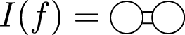
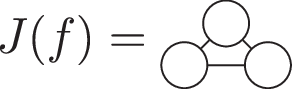
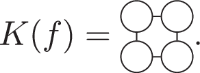
$$\begin{array}{lcl}I(f) & = & \mathop{\sum }\limits_{\alpha \beta }{f}_{\alpha \beta }^{2}{f}_{\alpha \beta }^{2}={\rm{T}}{\rm{r}}[{{\boldsymbol{f}}}^{2}\cdot {{\boldsymbol{f}}}^{2}]\\ J(f) & = & \mathop{\sum }\limits_{\alpha \beta \gamma }{f}_{\alpha \beta }^{2}{f}_{\beta \gamma }^{2}{f}_{\gamma \alpha }^{2}={\rm{T}}{\rm{r}}[{{\boldsymbol{f}}}^{2}\cdot {{\boldsymbol{f}}}^{2}\cdot {{\boldsymbol{f}}}^{2}]\\ K(f) & = & \mathop{\sum }\limits_{\alpha \beta \gamma \delta }{f}_{\alpha \beta }^{2}{f}_{\beta \gamma }^{2}{f}_{\gamma \delta }^{2}{f}_{\delta \alpha }^{2}={\rm{T}}{\rm{r}}[{{\boldsymbol{f}}}^{2}\cdot {{\boldsymbol{f}}}^{2}\cdot {{\boldsymbol{f}}}^{2}\cdot {{\boldsymbol{f}}}^{2}]\end{array}$$

(12)

Here, suitable for the ℓ = 2 tensor, $Tr[\ldots ]$ denotes the matrix trace operation and ⋅ the matrix multiplication operation. The order of the contraction indices does not matter because the tensors are symmetric. When considering tensors of varying ranks, we need not explicitly label ℓ for each tensor, because this is given by the number of indices. This allows us to associate invariant contractions with multigraphs, i.e., graphs where more than one edge may be associated with each pair of nodes, as follows:

(13)

(14)

(15)

This kind of diagrammatic representation, referred to as tensor diagrams or Penrose diagrams⁶⁹, has a variety of uses and is used to visualize moment invariants and remove redundancies⁷⁰. The graph captures the notion that the order of indices within tensors is irrelevant; edges need not be labeled. Tracelessness means that graphs with self-loops must be equal to zero, and can therefore be ignored. Another advantage of the graph approach is that it easily avoids examining invariants that factor into a product of lower-order invariants. In the graph formulation, this corresponds to a graph that has multiple connected components. This kind of redundancy has been identified previously by the authors of NICE in the spherical tensor formulation³³. In the present work, we shall consider primarily the invariants of a single function $f(\widehat{{\bf{r}}})$, and in this context, there is no need to label nodes; nodes with different degree ℓ correspond precisely to the tensor ${{\boldsymbol{f}}}^{\ell }$.

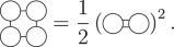
Similarly to ACE, sets of all Cartesian graph invariants scale combinatorially, and the problem of redundant invariants emerges even for simple cases such as the functions in Eq. (12). First, we consider regular graphs, i.e., graphs in which all nodes have the same number of edges. They correspond to pure invariants⁵⁴, i.e., invariants that are contractions of powers of a single irreducible moment tensor. It is well known that a traceless, symmetric 2-tensor contains only two invariant degrees of freedom, which can be seen from its eigendecomposition. Somewhat more algebra is required to identify the relation between the three second-rank pure graph invariants from (12), which is

$$K(f)=\frac{1}{2}I{(f)}^{2}$$

(16)

(17)

However, a matrix decomposition does not apply straightforwardly to rank ℓ = 3 tensors, and becomes conceptually more difficult for higher-rank tensors. Nonetheless, they also contain relations. An example relation among the set of ℓ = 3 graphs is

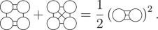
(18)

The ℓ = 3 tensor corresponds to a particular function on the sphere. There are manifestly 2ℓ + 1 = 7 components to this function; however, three degrees of freedom in these components determine the orientation of the function (parameterized, for example, by three Euler angles).

For regular graphs, all that is needed is to use the Langbein approach to identify graphs that contain functionally independent information until a set of 2ℓ − 2 invariants has been found. There are exceptions for the number of invariants for ℓ = 0 and ℓ = 1 owing to the reduced degrees of freedom necessary to orient scalars and vectors. In total, the number of pure invariants that can be extracted from the tensor representations up to an order ℓ is quadratic in ℓ. The complete theorems and a table summarizing the degrees of freedom of functionally independent invariants can be found in the companion paper. There it is also shown that no complete set can be generated using pure invariants only.

Finding information in the set of mixed invariants, i.e., contractions that contain tensors of differing rank, might appear to be a more daunting task, owing to the variety of non-regular graphs. However, with the pure invariants taken care of, the mixed invariants need only perform a simpler task: for each pair of orders ℓ and ${\ell }^{{\prime} }\ne \ell$, the mixed invariants only need to determine the relative orientation of the functions represented by ${{\boldsymbol{f}}}^{\ell }$ and ${{\boldsymbol{f}}}^{{\ell }^{{\prime} }}$, which requires at most three invariants. There are again exceptions to this count when one order ℓ is small; in particular, there are no independent mixed invariants involving ℓ = 0, which is in itself a graph, and only two degrees of freedom are needed to describe the orientation of a pattern relative to a vector (ℓ = 1).

Bujack et al. proved that a basis of invariants can be generated by taking all pure invariants, then choosing one order ℓ₀ whose moment tensor is guaranteed to be non-zero robustly across all admissible functions and adding three mixed invariants between it and each other tensor⁵¹. While such a non-zero tensor can be chosen in some pattern recognition applications, this is not possible in our application. For a function whose ℓ₀ tensor is zero, all mutual-orientation information is lost, and the basis is no longer complete. To reliably guard against the problem of a priori unknown vanishing tensors, one must include mixed invariants that connect all orders ℓ to all other orders ${\ell }^{{\prime} }$. This so-called minimal flexible set⁵⁴ is not a basis because it is not functionally independent. But it is the smallest possible set that is complete for any a priori unknown function. While this comes at the cost of a larger number of invariants, this scaling is quadratic and therefore asymptotically equivalent to any invariant basis for spherical functions.

The feature sets in practice

Even though these results guarantee optimal feature sets in theory, in practice, other criteria play a role. For example, descriptors vary in their evaluation speed. Further, descriptors with lower polynomial order—a function of the order of the moments and number of factors in the tensor product—are less prone to loss of precision in floating-point calculations.

One way to reduce the theoretically-optimal feature sets to feature sets that work efficiently and robustly in practice is by explicitly limiting the total invariant polynomial order, or the number of factors in the products, and using only the subset of the optimal set that falls below these limits. Alternatively, this limit can be applied before Langbein’s algorithm is executed. The advantage of this is that fewer candidates need to be tested. The disadvantage is that the stopping criterion is a priori unknown.

With these principles, analogously to the procedure in “A functionally-independent subset for ACE” section, we have performed a numerical search for a flexible set of Cartesian tensor invariants by enumerating graphs, constructing random tensors, and applying the Langbein test for independence; more information on this process is provided in “Search procedure for graph invariants” section. Table 5 lists a minimal flexible set up to a number of factors n = 4 and moment order ℓ = 3, which in this special case happens to be equivalent to limiting the total descriptor polynomial order to m = 12. The result includes one scalar graph, three tensor-norm graphs containing exactly two nodes each, two further pure invariants, and seven mixed invariants. This set can characterize all of the available information in a single function up to ℓ = 3 while using at most four terms in an invariant.

Table 5 Flexible invariant set of moment order ℓ = 3 reduced to n ≤ 4 terms

We use the minimal flexible set from Example 9 in the companion paper⁵⁴ and restrict it to a total descriptor polynomial order 12. This reduces the original complete set of eight pure invariants to six. The seven mixed invariants are not affected. This leads to a total of 13 invariants, which coincides with the size of a basis for these tensors.

This set of invariants is visualized in Fig. 4. Here, an input set of tensors was selected to maximize the orthogonality of the invariants. Details of this procedure are given in the Supplementary Note 2. This yields a pattern on the sphere, and gradient patterns on the sphere describing the direction of change for each invariant. The gradient for invariant 0, which is always a constant function, is omitted. With the exception of invariants 4 and 5, which are similar (but still mathematically independent), the invariants selected correspond to a broad set of patterns. Thus, each invariant serves to recognize different modalities of change to the input function. It is important to recognize that this input pattern is not unique, as it is the result of optimization over the nonlinear invariants.

Incorporating flexible bases into atomistic neural networks

We start with the general form of the HIP-NN interaction layer, first introduced in ref. ²⁰. Atomic features z_i,a, where i indexes atoms and a indexes features, are transformed using the functional form

$${{z}^{{\prime} }}_{i,a}=f\left({{\mathcal{I}}}_{i,a}(z,{\bf{r}})+\mathop{\sum }\limits_{b}{W}_{ab}{z}_{i,b}+{B}_{a}\right).$$

(19)

The weight matrix W_ab describes a feature transformation that is local to each atom between features a and b, with a bias vector B. The activation function f acts point-wise on each element. The interaction function ${\mathcal{I}}$ specifies how features in the environment can affect a particular atom i. This form is rather general, and with specific functional forms for ${\mathcal{I}}$, one can arrive at many kinds of models from the literature. In HIP-NN, the interaction function is an explicit product of a radial representation s^ν(r_ij) and the features z_j on neighboring atoms with a learnable weight tensor (in the multi-dimensional array sense) ${V}_{ab}^{\nu }$:

$$\begin{array}{rcl}{{\mathcal{I}}}_{i,a}{(z,r)}^{{\rm{H}}{\rm{I}}{\rm{P}}-{\rm{N}}{\rm{N}}} & = & \mathop{\sum }\limits_{j}{m}_{ij,a}\\ & = & \mathop{\sum }\limits_{j,b}{v}_{ab}({r}_{ij}){z}_{j,b}\\ & = & \mathop{\sum }\limits_{j,b,\nu }{V}_{ab}^{\nu }{s}^{\nu }({r}_{ij}){z}_{j,b}.\end{array}$$

(20)

Here we define an intermediate message m_ij,a, sent from neighbor j to atom i on feature index a, as well as a variable weight function v_ab(r_ij), with r_ij = ∣r_i − r_j∣. To expand on this framework to include directional information, it is natural to consider an environment function ${{\mathcal{E}}}_{i,a}(\widehat{{\bf{r}}})$ which represents the messages received by an atom at any direction $\widehat{r}$

$${{\mathcal{E}}}_{i,a}(\widehat{{\bf{r}}})=\mathop{\sum }\limits_{j}\delta (\widehat{{\bf{r}}}-{\widehat{{\bf{r}}}}_{ij}){m}_{ij,a}.$$

(21)

The message distribution can be broken down into irreducible tensor components using irreducible tensors T^ℓ of Eq. (10). This generates environment tensors as projections of the environment function onto each Cartesian irreducible tensor:

$${\boldsymbol{\mathcal{E}}}_{i,a}^{\ell }=\int {{\bf{T}}}^{\ell }(\widehat{{\bf{r}}}){{\mathcal{E}}}_{i,a}(\widehat{{\bf{r}}})\,{d}^{2}\widehat{{\bf{r}}}.$$

(22)

In this notation, the original HIP-NN interaction is simply a single term in a series of environment tensors:

$${{\mathcal{I}}}_{i,a}^{HIP-NN}={\boldsymbol{\mathcal{E}}}_{i,a}^{0}.$$

(23)

A second class of HIP-NN models, called HIP-NN with Tensor Sensitivities, or HIP-NN-TS, was introduced in ref. ³¹, which mixes environment tensors of different orders ℓ by taking their norms and mixing parameters ${t}_{a}^{\ell }$:

$${{\mathcal{I}}}_{i,a}^{HIP-NN-TS}={\boldsymbol{\mathcal{E}}}_{i,a}^{0}+{t}_{a}^{1}| {\boldsymbol{\mathcal{E}}}_{i,a}^{1}| +{t}_{a}^{2}| {\boldsymbol{\mathcal{E}}}_{i,a}^{2}| +\ldots \,.$$

(24)

This same ansatz—that the tensor norms provide a useful but far cheaper subset of the full tensor information—was also used by SO3KRATES^39,40. We now turn to the question of a strategy to integrate the invariants of the “Cartesian formulation of tensors and enumeration of invariants as graphs” section into a similar neural network architecture. Now, with a set of invariant functionals ${{\mathbb{I}}}^{k}[\cdot ]$ which are indexed by k, operating as functions of the tensor components of the function as ${{\mathbb{I}}}^{k}({\boldsymbol{\mathcal{E}}}^{0},{\boldsymbol{\mathcal{E}}}^{1},\ldots \,)$, we can consider a set of scalar features ${{\mathbb{I}}}_{i,a}^{k}$ generated by these functionals:

$${{\mathbb{I}}}_{i,a}^{k}={{\mathbb{I}}}^{k}[{{\mathcal{E}}}_{i,a}(\widehat{{\bf{r}}})].$$

(25)

That is, the invariants are applied channel by channel, similarly to the tensor sketch as outlined by Darby et al.⁷¹. The invariants operating channel-wise do not heavily constrain the interaction because these channels are already parameterized mixtures of the underlying features z, mixed using the tensor ${V}_{ab}^{\nu }$ of Eq. (20). This is evident by performing the integration over the sphere and expanding the definition of ${\boldsymbol{\mathcal{E}}}_{i,a}^{\ell }$ in terms of scalar components:

$${{\mathcal{E}}}_{i,a,\overrightarrow{\alpha }}^{\ell }=\mathop{\sum }\limits_{j,b,\nu }{V}_{ab}^{\nu }{T}_{\overrightarrow{\alpha }}^{\ell }({\widehat{{\bf{r}}}}_{ij}){s}^{\nu }({r}_{ij}){z}_{j,b},$$

(26)

where $\overrightarrow{\alpha }=({\alpha }_{0},{\alpha }_{1},…,{\alpha }_{\ell -1})$ represents the ℓ Cartesian indices associated with a rank-ℓ tensor. We choose these functions ${\mathbb{I}}$ to be a flexible set of invariant polynomials in accordance with the search from the “Search procedure for graph invariants” section. This set is indexed by two hyperparameters: the maximum value of ℓ used, and the maximum polynomial order n.

While these features are scalar, and it is possible to use them in an arbitrary neural network layer, early experiments demonstrated a difficulty with handling especially high-order invariants. The difficulty is that the order of magnitude of high-order invariants can easily be larger or smaller than those of low-order invariants; a fourth-order polynomial can easily have a magnitude far higher or lower than a 2nd order polynomial. Naturally, the magnitude of the environmental features will vary in varying environments, and as such, changes in the magnitudes of the tensors will have a far greater effect on the magnitude of higher-order invariants than lower-order ones. A remedy to this is group normalization, or GroupNorm, which adjusts groups of activations relative to their own mean and standard deviation⁷². We therefore apply group normalization where each group corresponds to its own invariant graph, k, across the features, a, to compensate for the effect of different invariants being larger or smaller, yielding activations ${\widetilde{{\mathbb{I}}}}_{i,a}^{k}$:

$${\widetilde{{\mathbb{I}}}}_{i,a}^{k}=GroupNorm < k > ({{\mathbb{I}}}_{i,a}^{k}).$$

(27)

We then mix these features to define a new interaction function. Quantitative results on the effectiveness of GroupNorm are presented in the “Results” section and in Supplementary Note 6. Because the flexible set of invariant polynomials makes feasible the computations at greater body-order, we refer to this new version of HIP-NN using high-order polynomials as HIP-HOP-NN:

$${{\mathcal{I}}}_{i,a}^{HIP-HOP-NN}=\mathop{\sum }\limits_{b,k}{{\mathbb{W}}}_{ab}^{k}{\widetilde{{\mathbb{I}}}}_{i,b}^{k}.$$

(28)

Search procedure for graph invariants

The search for independent graph invariants proceeds as follows: The root loop covers the sectors of invariants; a sector being the set of tensors used in the polynomial. The (1,) sector is the space of homogeneous polynomials using only the order ℓ = 1 tensor, and the (1, 2) sector is the space of heterogeneous polynomials using both the order 1 tensor and the order 2 tensor. Within these sectors, based on the counting of degrees of freedom in ref. ⁵⁴, the number of possible independent invariants is well-determined; the homogeneous sectors contain ℓ − 2 independent invariants and the heterogeneous sectors contain at most 3 invariants independent from the homogeneous ones. Finding this many independent invariants in each sector delineates a flexible set of invariants.

Now, within a sector, the loop covers the space of the invariant terms in the final polynomial; for example, a term 1²2² represents a polynomial coupling two factors of the order 1 tensor with two factors of the order 2 tensor. These terms are searched in an ascending order of the total number of factors. For mixed invariants, terms involving lower-order invariants are searched before higher-order invariants (e.g., 1²2¹ is searched before 1¹2²).

Within a term, the set of scalar tensor contractions is enumerated. This proceeds by assigning pairs of edge indices to each tensor in the term in an ordered fashion. As the enumeration proceeds, if the partial terms already assigned form a connected graph, then the subsequent index permutations are discarded; otherwise, the final index assignment will form at least two disconnected components. Furthermore, as each tensor term is assigned indices, the topology of the partial graph is analyzed and compared against previously visited graphs in the same terms. The comparison is done using NetworkX⁷³ first with the Weisfeiler-Lehman (WL) graph hash for fast isomorphism rejection. If the present graph does have the same WL hash as a previously visited graph, then it is further examined using full isomorphism testing. Previously explored partial-graphs are discarded immediately, preventing the need to search down many branches of the enumeration tree of tensor contractions.

As enumerated contractions are yielded from this procedure, they are tested for independence against the current set of independent invariants. This is done using random values for each tensor in the sector; the components of each of which were uniformly distributed from 0 to 1. Then the values of the invariants, the subsequent Jacobian, and the rank of the Jacobian were calculated using PyTorch⁷⁴ autograd features. If the rank of the Jacobian increases by the addition of the yielded invariant, it is added to the set of retained independent invariants. The search is terminated if the number of invariants in the retained set is equal to the degrees of freedom available within a sector, or all terms in that sector up to the given factor cutoff n have been searched.

Training details for methane configurations dataset

The same model hyperparameters were used for each network type and training set size. Each model has one interaction layer, three atom layers with 32 features each, and 20 sensitivity functions. A starting batch size of 256 was used, and the batch size was doubled up to three times if 150 epochs passed without any improvement to the energy MAE on the validation data, as suggested in ref. ⁷⁵. The Adam optimizer⁷⁶ was used with a learning rate of 2.5 × 10⁻³. Training was terminated if 300 consecutive epochs passed with no improvement to the energy MAE on the validation data or if a total of 10,000 epochs elapsed. The hyperparameters were selected with the aim of creating models that could be quickly trained, so that the 440 total models could be trained while allowing enough expressivity that the models could learn well. The models were trained to match both forces and energies associated with the configurations.

Hyperparameter search methods for QM7 models

The hyperparameter search for the QM7 models was performed using a Tree-structured Parzen Estimator⁷⁷, a Bayesian optimization method frequently employed for hyperparameter tuning. The search was implemented with Ray Tune⁷⁸ and Hyperopt⁷⁹. There were 200 trials conducted for each network type, with the results for each trial being an average from 10 trained models on a specific set of hyperparameters. The search space consisted of seven hyperparameters, the best found combinations of which are listed in Table 6. Each model was trained using a random 70% of the QM7 dataset. An additional 10% was used to measure early-stopping criteria for model training and to quantify model performance for the hyperparameter search. The remaining 20% in each case was not used during the hyperparameter search. The results in Table 1 are calculated from 10 models using the best hyperparameters found for each network type, again using a random 70 + 10% of the QM7 data. The MAE and RMSE values reported in the table are on the final 20% of the data. An example code for performing this hyperparameter search can be found in the open-source hippynn⁸⁰ repository, which implements the HIP-NN family of models.

Table 6 Best hyperparameter set found for each model for the QM7 dataset

Hyperparameters for QM9 and ANI-1x HIP-HOP-NN models

The HIP-HOP-NN hyperparameters used for the QM9 dataset and ANI-1x dataset are shown in Table 7. The ANI-1x model is also used for the speed tests in this work. For more details about the hyperparameter setup, see ref. ³¹.

Table 7 The HIP-HOP-NN hyperparameters used for the QM9 and ANI-1x benchmark problems

Force training schedule for QM9

The QM9 dataset contains equilibrium structures with zero values for all force components. These forces can be added to the training protocol for MLIPs to improve the modeling of energies. The force weighting in the loss function is set to 1 for the first 10 epochs, 2 for 50 epochs and then 0.1 for the remaining training.

Source link