Explainable machine learning with bayesian hyper-optimization for predicting cognitive impairment from longitudinal nursing home data

Dataset

The dataset used in this study originates from a retrospective cohort of residents from four DomusVi nursing homes in Spain. Ethical approval for the study was granted by the relevant institutional committee (Code: 2023/576). The database contains information from 2,608 residents and includes 4,718,828 activity records collected over a 13-year period (2011–2024). Each entry is time-stamped, enabling longitudinal tracking and reconstruction of monthly follow-up periods. The dataset is a proprietary clinical resource generated as part of routine care activities at DomusVi and is not publicly available due to institutional and privacy constraints. Access for research purposes was provided under the approved ethics protocol. All methods were carried out in accordance with relevant guidelines and regulations, including the Declaration of Helsinki and institutional policies governing research with human participants. Written informed consent was obtained from all participants or their legal guardians prior to data collection, following institutional and national ethical standards.

The information is organized into nine IS capturing different dimensions of residents’ health and daily activities, such as clinical variables, medication prescriptions, nutrition, bowel movements, falls, and activity logs. Each IS contains heterogeneous variables with distinct sampling frequencies. Table 1 summarizes the number of records per IS. The use of timestamps across all entries facilitates alignment of the disparate data streams along a common temporal axis for harmonized longitudinal analysis.

Demographics (Subjects IS)

The Subjects IS contains a unique identifier for each resident, along with gender, age at entry, and follow-up duration. Table 2 presents summary statistics (mean, standard deviation, minimum, and maximum) for the overall cohort and stratified by gender (998 males and 1,610 females).

Clinical variables IS

This IS includes 40 clinical variables recorded during follow-up, totaling 414,219 entries. Some variables were measured frequently, while others had sparse entries. This IS also includes the Tinetti and Mini Nutritional Assessment (MNA) (determinate for three variables: MNA_Global_score, MNA_Assessment_score and MNA_Screening_score) scores that measure the functional mobility and nutritional status of individuals, respectively.

Bowel movement records IS

This source contains 3,948,306 daily records. Each entry includes time of day (morning, afternoon, evening) and one of seven stool classifications: X (no movement), N (normal), D (diarrhea), B (soft), F (impaction), L (liquid), and E (constipation).

Fall records IS

With 8,228 entries, this IS captures categorical data about fall events. See the Supplementary Material S2 table for the whole description of categorical variables. Such categorical variables include the following content, describing the episode as: accompaniment during the fall (Id_AccompanimentFall), conduct to follow (Id_ConductToFollow), associated symptom (Id_AssociatedSymptom), and type of injury caused by the fall (Id_TypeOfInjuryFall). Additionally, this IS includes variables for the location of the fall (Id_FallLocation), cause of the fall (Id_CauseFall), neurological state (Id_NeurologicalState), and activity (Id_ActivityFall) along with the timestamp of the event. If the resident has no falls, there are no inputs in this IS.

Drug prescriptions IS

This IS comprises 273,679 records of medication administration, specifying drug name, dosage, frequency, and administration start and end dates.

Nutritional plan S

The Nutritional Plan contains 48,875 records detailing the start and end dates of each resident’s dietary plan. Each record includes the plan identifier (Id_Diet), calories information (Id_Calories), route of administration (Id_Route), and consistency (Id_Consistency). For subsequent analysis, only meals categorized as breakfast, lunch, snack, and dinner are included. Using this criterion, 46,565 determinations from the table will be analyzed.

Cognitive impairment scales IS

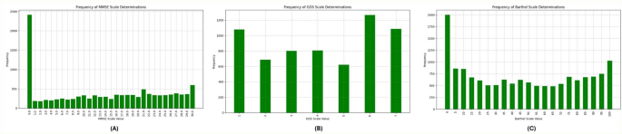
The Cognitive Impairment Scales contains the determinations of CI using three different scales, namely MMSE scale, Barthel scale and GDS scale for each resident, describing their condition throughout the follow-up study. The number of determinations for each scale varies, as evidenced by the values in Table 1, with an average of 2.08 determinations per patient for MMSE, 1.37 determinations per patient for GDS, and 2.57 determinations per patient for Barthel. The distribution of the frequency for each scale’s values is provided in Fig. 1, illustrating the prevalence and severity of CI among the study participants over time. It is remarkable that the number of determinations with MMSE = 0 corresponds to residents that are not able to undergo the test.

AI tools (predictors and explainability)

ML predictors (Bayesian Hyper-optimized XGBoost predictors)

XGBoost²⁰ is a Boosting technique within Ensemble Learning, designed to enhance prediction accuracy by combining multiple models. Unlike other boosting methods that increase the weights of misclassified examples, XGBoost optimizes a loss function through gradient boosting. Its objective function, optimized at each iteration, is given by Eq. 1.

where, \(\:l\) represents a differentiable convex loss function, \(\:{(x}_{i},{y}_{i})\) is the training set, \(\:{\stackrel{\sim}{y}}_{i}\) is the final prediction, and \(\:\varOmega\:\left(ft\right)\) is the regularization term that prevents overfitting by penalizing complex models using Lasso and Ridge regularizations.

XGBoost constructs the next learner by maximizing loss reduction, using the Exact Greedy Algorithm. This process starts with a root node containing all training examples, evaluates potential splits for each feature, and stops growing a branch if the gain for the best split is not positive. Setting up XGBoost involves three types of parameters: general, booster, and learning task parameters. General parameters define the booster type (tree or linear model), booster parameters configure the internal aspects of the booster (like learning rate and number of estimators) and learning task parameters specify the learning objective.

Bayesian hyper-optimization enhances ML predictors, including XGBoost, by systematically optimizing hyperparameters for maximum model accuracy²¹. It uses Bayesian inference to balance exploration and exploitation in the hyperparameter space, making the search more efficient than traditional methods like grid or random search. By defining a probabilistic model of the objective function and updating it with new data points, Bayesian optimization quickly identifies the most promising hyperparameter regions, thus speeding up training and improving generalization. For XGBoost, this involves tuning parameters like learning rate, maximum depth, and subsample ratio, which are iteratively adjusted based on validation set performance. This results in a robust model with superior predictive accuracy and reliability, making Bayesian hyper-optimized XGBoost predictors a powerful tool in ML²².

Shapley additive explanations (SHAP)

SHAP is a powerful tool used in explainable AI to reveal the importance of input features in model predictions¹⁸. It applies principles from game theory to quantify the contribution of each feature to the model’s outputs. By considering all possible combinations of features, SHAP provides insights into how these features interact and collectively influence predictions. Equation 2 represents the mathematical expression of SHAP values. This comprehensive approach enhances transparency in complex ML models, enabling informed decision-making regarding feature importance and model behavior. Equation 2 represents the mathematical expression representing SHAP values.

where (S) represents the output of the XGBoost model based on a particular subset of features, denoted as S, from the complete set N of all features. The contributions (\(\:{\varnothing\:}_{i}\)) are determined by averaging the impacts across all possible permutations of feature sets. As each feature is sequentially added to the set, its influence on the model’s output change becomes apparent.

Methodological framework

In this work, we present a comprehensive framework employing AI predictors (regressors and classifiers) based on XGBoost algorithms, using both default parameters and Bayesian hyper-optimization to construct AI predictors of CI. This framework allows to evaluate the informative contribution of various IS within a heterogeneous dataset on the living conditions of elderly individuals in nursing homes, addressing the outlined problem. Finally, by employing SHAP to comprehend the reasons behind such predictions, we aim to gain a better understanding of the CI process. The general schema of the methodology developed in this work is depicted in Fig. 2.

The proposed method requires the recodification of the heterogeneous information collected from residences to create longitudinal models in a suitable homogeneous format. After this, the framework will enable the production of a family of predictors P_ijk from X_i datasets, which are created from i IS, j outcome variables that define clinical questions (y_j), and k sets of hyperparameters for ML algorithms that generate possible models. The parameter k can iterate over different ML algorithms and various sets of hyperparameters for each algorithm. In this work, for simplicity, we propose reducing the ML algorithm to XGBoost¹⁹, used as a regressor and classifier. We propose using the information from the Subjects (Residents) IS in combination with each of the other tables (Fall Records, Clinical Variables, Bowel Movement Records, Drug Prescriptions, and Nutritional Plans) to form the Xi​ datasets and create combinations to predict the yj (MMSE, GDS, and Barthel scales). After identifying the best predictor (according to the AUC metric for regressor), the explicability stage will help in identifying the reasons behind the decisions made.

Thus, the methodology consists of three main steps: the first focuses on recoding data to transform the heterogeneous information of each individual into a homogeneously structured matrix and make it possible to use the dataset on the family of Pijk predictors. The second step identifies the best predictors for specific clinical outcomes. The final step employs XAI to understand the rationale behind the model’s decisions of Pijk. In this way, the methodology allows us to run experiments to elucidate the importance of each data source for predicting the CI, as presented previously.

Data recodification

The first step is to merge all the IS to create a single time axis that contains all the collected information. To produce a homogeneous dataset from the longitudinal multidisciplinary IS, the proposed schema for analysis requires reshaping the data into a new format, as illustrated in Fig. 3. In this paper, we propose a monthly-based recodification where data for each resident are organized monthly for both Xi and yj variables.

The number of determinations of clinical events over time varies greatly and occurs without a temporal pattern, except for Bowel Movement Records and Nutritional Plans, which are recorded three times daily (morning, afternoon, and evening) and four times daily (breakfast, lunch, afternoon snack, and dinner) respectively. To conduct the monthly analysis, different considerations are taken depending on whether the variable describing the event is categorical or numerical. For the recording of the categorical determinations of daily bowel movements, the number of occurrences of each reference value is accounted for the entire month in each period. This leads to a reduction of data into 21 variables, representing three time periods (morning, afternoon, evening) across seven categories, with each variable representing the number of monthly occurrences. For the Fall Records IS, the monthly number of falls is logged along with the associated information for eight variables, as described in Dataset section.

In the case of the Drugs Prescription IS, the days of the month on which each medication is taken are recorded, along with the active ingredient and corresponding dose. If multiple medications are taken, the same procedure is followed, associating each medication with the patient’s monthly record. This produces a monthly vector of variable length for each resident, depending on the number of medications administered. To obtain a fixed-length vector computationally, the principle of one-hot encoding can be used²³. This algorithm produces/encodes as many columns as possible medications to be administered, producing a triple description for each (in terms of the active ingredient, dose, and frequency, using zero for the drugs not consumed in that month period).

In the case of the Clinical Variables IS, if there are multiple measurements within a month, the average, standard deviation, minimum, and maximum values are extracted. For the Tinetti and MNA scores, the measured value within a 3-month period is retained. Since several variables have empty values, indicating the absence of data for those variables in certain months, it is necessary to use a filling parameter (FP). The FP represents the proportion of non-empty values for each variable, providing insight into how thoroughly each variable is documented within the dataset. Figure 4 illustrates the FP for variables of Clinical Variables IS. The variables are listed on the x-axis, while the FP percentage is on the y-axis. From the figure, we observe that variables such as the MNA Score, Tinetti Score, and blood pressure (systolic and diastolic) have a high FP, nearing 100%. This indicates that these variables are almost always recorded. Other variables, such as Weight, BMI, and Heart rate, also show relatively high FPs above 60%, represented by a dashed green line indicating the 50% threshold. In contrast, many variables have significantly lower FPs, indicating that they are less frequently documented. The low FP of these variables suggests that they might not be consistently available for analysis, which could impact the comprehensiveness of any study relying on this data.

Before data monthly-basis, it is essential to ensure continuity for the discontinuous variables that require prediction, namely MMSE, GDS, and Barthel. In this study, we propose utilizing the most recent recorded value until a new determination is documented, within a 3-month period^24,25.

Building predictors for CI scales (P
_ijk)

Given a homogeneous dataset, as the monthly-based harmonized data produced in Data recodification section, the problem of identifying the amount of information in each IS of the dataset, can be posed in a general manner as identify the parameters of a family of predictors Pijk, that can be regressors or classifiers, depending on the underlying clinical problem associated with the output variable yj. In a general manner approach, given a homogeneous dataset X = Xi, it can be understood as a joining of variables from n different IS, to predict (regressing or classifying) j outcomes variables y = yj. Examples of this outcome proposed in this work are the prediction of the CI scales, presented in Dataset section. In this work we propose to use XGBoost¹⁹ as predictor and use default parameters and Hyper-opt, which uses Bayesian methods²⁰ to optimize the search of the k sets of parameters. The method allows us to identify the set of parameters that provides the best performance in the prediction of j clinical questions. Each predictor will have a performance metric.

Using the monthly-based IS of residents, it is possible to predict CI scores described above (MMSE, GDS and Barthel). These predictors can be used as a measurement of the predictive value of the dataset.

Given the longitudinal and patient-centered nature of the dataset, standard random splitting would lead to information leakage and artificially optimistic performance. To prevent this, we implemented a nested cross-validation (nested CV) scheme with grouping and temporal constraints. A 5-fold outer cross-validation loop was used to estimate generalization performance. All monthly observations from a given resident were assigned to the same fold to avoid leakage across folds. In addition, within each resident, temporal ordering was preserved to ensure that training data always preceded test data chronologically. Inside each outer training fold, we performed a 3-fold inner cross-validation loop to select hyperparameters through Bayesian optimization (Hyperopt). The inner loop searched for the hyperparameter space using only the training folds of the outer loop. The best hyperparameters obtained in the inner loop were then used to fit a final model on the entire outer training set and subsequently evaluated on the corresponding outer test fold. This nested design ensures (i) unbiased estimation of the true generalization error, (ii) rigorous separation between hyperparameter tuning and model evaluation, and (iii) protection against patient-level and temporal leakage ― all of which are essential for real-world longitudinal clinical data.

Artificial intelligence explainability (XAI)

Once the predictor models are built it is possible to employ XAI tools to analyze the black box. The final predictor Pijk can be explained using the SHAP approach¹⁸. In this methodological stage information of the importance of the variables is obtained as well as the explanations of the role that the variables play on predictions.