High-entropy advantage in neural networks’ generalizability

Arithmetic Question

We began our investigation with small fully-connected neural networks (FNNs) on a relatively simple arithmetic task: learning a predefined equation of binary classification. Here we constructed a synthetic Spiral Classification Dataset, where every data entry is a point on 2-D space with a color (brown or green) determined by its coordinates. We generated 20 green points and 20 brown points randomly, forming two spirals. Our task is to predict a point’s color given its coordination. Therefore, this is a binary classification problem with 2 input features (horizontal and vertical coordinates). More details, including the equation used and visualization of this synthetic dataset are presented in the Methods section.

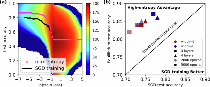
We used Wang-Landau Monte Carlo (WLMC) method to sample the entropy landscape, S(L_train, A_test), as a function of the log-scaled train loss, \(ln({L}_{train})\), and test accuracy, A_test. The log-scaled train loss allows us to better sample the low L_train states, corresponding to trained NNs. In Fig. 1a, we present the entropy landscape for a (3 layers) × (6 neurons) FNN (116 trainable parameters). Warmer color represent higher entropy. The WLMC method (and the Wang-Landau Molecular Dynamics method we will employ later) calculates the entropy with an algorithm-dependent zero point; thus, the absolute value of the entropy lacks physical significance, but the entropy difference between any two points in Fig. 1 (a) carries physical meaning. For each given \(ln({L}_{train})\), we can calculate the corresponding equilibrium test accuracy:

where S is the entropy and a is variable standing for the test accuracy. 〈A_test(L_train)〉 are plotted as magenta dots in Fig. 1a and we refer it as the equilibrium accuracy in this paper.

We then performed classical training via the SGD optimizer for 100 times and collected the L_train versus A_test trajectories. For each given L_train, we calculated the mean A_test, which is plotted as the black curve in Fig. 1a. For simplicity, we refer it as the SGD accuracy in this paper. We can see that when L_train reaches a low level [\(ln({L}_{train})\approx -0.5\))], the equilibrium accuracy increases rapidly with the decrease of L_train and gets saturated when \(ln({L}_{train})\approx -3\). In this regime, we observed a supremacy of the equilibrium accuracy over the SGD accuracy for each given \(ln({L}_{train})\), which indicates the existence of high-entropy advantage. Another interesting observation is that when the training loss is at a high level (\(ln({L}_{train}) > 0\)), the equilibrium accuracy is around 50%. This also agrees with intuition, because when a FNN has a high L_train, the highest-entropy state of the model is just making random guesses, which results in 50% accuracy for binary classification.

We followed the same protocol and further tested on 3 additional FNN sizes and 2 different training time (total 8 experiments, see more details in Supplementary Information). Results are presented in Fig. 1b. For all experiments, the training loss at the end of SGD training corresponds to an equilibrium test accuracy that outperforms the SGD accuracy with a large margin, further verifying that the high-entropy state can provide better generalization. The smallest FNN tested here (3 layers × 6 neurons) has 116 trainable parameters, which is still much larger than the number of training data points, 40, guaranteeing the overparamterized nature of all models.

Kaggle House Price Prediction

After showing that high-entropy state can consistently provide better generalization for small FNNs, we then further extend the experiments to larger neural networks on real world tasks. Due to the increase of parameters number in large networks, WLMC becomes inefficient, as it has a time complexity of \({\mathbb{O}}(n)\) to update one parameter, where n is the total number of NNs’ trainable parameters. Therefore, we employed the Wang-Landau Molecular Dynamics (WLMD) method, which updates all n parameters together in each time step with time complexity \({\mathbb{O}}(n)\). (See Methods for more details)

We started from the House Price dataset²⁸ on Kaggle website²⁹, where the task is to predict the the house price from its descriptors like number of bedrooms and house age. For the sake of computational cost, here we only used the original training dataset which consists of 1460 houses. Each house has 79 descriptors (excluding the house ID) and we performed one-hot encoding for all categorical descriptors, yielding a total of 331 descriptors/features for each data point eventually. We randomly select 50% data as the training set, with the remaining data reserved for testing. A 2-layer FNN is used for this regression task, where the hidden layer has 20 neurons. Therefore, the final model has 6661 trainable parameters, making it overparamterized.

Following the similar protocol described above for the arithmetic question, we computed the entropy landscape, S(L_train, L_test), as a function of train loss, L_train, and test loss, L_test. Results are presented in Fig. 2a, where both L_train and L_test are on a log scale for clarity in the low-loss regime. In statistical physics, the probability distribution over different states (different locations in the plot) is sharply peaked around the entropy maximum, making the max-entropy state thermodynamic equilibrium. Therefore, we locate these max-entropy states at each L_train (magenta dots), and compare with SGD-trained states (black curve). SGD training results are averaged over 100 independent training instances using optimized hyperparameters, yielding error bars smaller than the black curve’s width. Our results suggest that at a given L_train, the corresponding max entropy loss is clearly lower than the test loss obtained via SGD training, demonstrating the high-entropy advantage in NNs generalizability. More technical details, including data and hyperparameter tuning, are presented in the Methods section.

MNIST Image: Handwritten Digit Recognition

Modern neural networks have demonstrated remarkable success in computer vision¹¹. One of the fundamental datasets used in the computer vision benchmark is the MNIST dataset, which consists of images of handwritten digits³⁰. Here we used it to further verify that the high-entropy advantage exists for the computer vision task. Since many models have achieved 100% accuracy on the test set of MNIST (see Leaderboard of Kaggle Digit Recognizer competition³¹), we strategically increase the difficulty of the MNIST task by a 200 times reduction of the training dataset size. This is done by randomly sampling 500 images from the original dataset and dividing them equally as the train and test sets, respectively. We refer this dataset as the selected MNIST dataset in this paper. The increased difficulty allows us to better observe the potential advantage of the high-entropy states. We built a small convolutional neural network with 5 convolutional layers followed by one fully-connected layer. This network has 362 trainable parameters, which is larger than the training dataset (250 images) in the selected MNIST, making it overparamterized.

In Fig. 2b, we presented the entropy landscape, \(S({L}_{train},{A}_{test}^{s})\), of this neural network on the selected MNIST dataset. Here \({A}_{test}^{s}\) is smoothed accuracy which is differentiable, as required by the WLMD algorithm (See Methods for details). We then find the max-entropy spot for each train loss on the landscape, which is again plotted as the magenta dots. Similar to the landscape in Fig. 1a, we observed an increase of max entropy test accuracy when the train loss reaches a low level [\(ln({L}_{train})\approx -1\)] and saturation at \(ln({L}_{train})\approx -4\). When the train loss is high, we observed a high-entropy band around the test accuracy of 0.1. This also meets our expectation because random guesses for this 10-class classification problem have an accuracy of 10%. We then performed classical training via the SGD optimizer for 200 times. (See more details in the Methods section.) The mean SGD accuracy are plotted as the black curve. Our results suggest that for a given train loss, the corresponding max-entropy states generalize better than SGD-trained states, especially when the train loss is small [\(ln({L}_{train}) < -2\)].

In order to confirm the existence of the entropy advantage in deeper neural networks, we investigated a 10-layer ResNet¹¹ (43604 trainable parameters) on a selected CIFAR-10 dataset (5000 images, equally divided for training and testing). The results, presented in the Supplementary Information, exhibit strong high-entropy advantage as well.

Polymer SMILES: Language Modeling

Natural language modeling is another domain where neural networks have consistently outperformed traditional machine learning methods^2,3,4. Language modeling also inherently differs from other machine learning tasks due to its reliance on semantic complexity and contextuality³². Therefore, we further extended our tests to a language modeling task. Specifically, we focused on a new emerging class of models called Chemical Language Models, which are language models trained on large databases of SMILES (Simplified Molecular Input Line Entry System)³³ strings and present promising performance in both predictive and generative tasks^34,35. We utilized the TransPolymer model published recently, which achieves state-of-the-art performance in all ten different downstream tasks for polymer property prediction³⁶. TransPolymer is a BERT (Bidirectional Encoder Representations from Transformers) family model^3,37 and is pretrained on roughly 5 millions polymer SMILES augmented from the Pl1M database³⁸. This pretrained transformer-based language model is able to take the SMILES as input directly and generate a 768-dimension embedding for each given SMILES. The embedding is then fed into a regressor head, a fully-connected layer with SiLU activation function, and is regressed on different polymer properties. Here we choose the Egb Dataset^36,39 to perform the entropy advantage experiment, which is the bandgap energy of bulk polymer and consists of 561 data points. This is also the dataset where TransPolymer has the best performance (test R² = 0.93), therefore, we can verify whether entropy advantage still exists for such a well-learned task. 80% data is used for training and the remaining 20% data is reserved for testing, which is same as the way reported in the original TransPolymer paper³⁶.

For sampling efficiency, we follow the fintuning strategy of large foundation model^36,40,41, where the encoder embedding is fixed and only tuning the regressor head of the TransPolymer model. We also reduced the width of the regressor to 50 while keeping the SiLU activation function. Therefore, the final model has 38501 parameters, making it overparamterized. Entropy landscape of this language modeling task is presented in Fig. 2c. The SGD training curve is obtained by performing the classical training for 40 times. As a regression problem, we found that the corresponding max-entropy loss at each L_train is slightly lower or comparable to its SGD training analog, which suggests that high-entropy state can generalize well. In other words, even for a task that could be well-learned via the SGD training, there is still a high-entropy advantage.

Effect of Network Width

Now that we have demonstrated high-entropy advantage in four distinct machine learning tasks, we will next study how this advantage is affected by the size of the neural network. It is known that neural networks are equivalent to Gaussian processes in the limit of infinite width^27,42. Therefore, it is reasonable to expect that the high-entropy advantage could also vary with the network width.

To better evaluate this, we constructed a Spiral Regression Dataset (see the Methods section for details) which consists of 500 data points and is divided equally for training and test sets. Using the same WLMD method, we sampled the entropy landscapes on NNs with 2 hidden layers of four different widths, W, ranging from 30 to 1000. All four models are overparamerterized and the largest one has more than 1 million trainable parameters. Our results, presented in Fig. 3, suggest that the high-entropy advantage decreases as W increases, and finally fades away when W = 1000. Note here we used the Adam optimizer here because the SGD optimizer performs much worse. We also performed similar experiments on the Kaggle House price prediction, the selected MNIST image recognition, and the Polymer SMILES language modeling tasks. These additional experiments confirmed a similar trend: the high-entropy advantage is more significant for narrower networks (see Figures 3–5 in the Supplementary Information).