Understanding how destination attributes shaping tourist visitation on cultural routes through social media data and interpretable machine learning

Study area

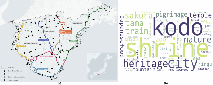
The study takes the Kumano Kodo in Japan as a case, one of the most representative cultural routes worldwide. The route consists of multiple historical paths with over 1000 years of history—including the Kiiji, Nakahechi, Kohechi, Ohechi, Iseji routes and Omine Okugakemichi (Fig. 1a)—which once connected Kyoto and Nara with the three Grand Shrines of Kumano. Originally functioning as a pilgrimage system, the routes attracted emperors, nobles, and monks, and hold significant cultural and spiritual value²⁹. Today, the Kumano Kodo has developed into a popular tourism destination whose appeal extends far beyond pilgrimage. TF–IDF analysis of English X posts from 2010 to 2025 shows that tourists associate the route with a wide range of themes, including Japanese shrine, train transportation, urban landscape, sakuragari, mountain scenery, hiking, Japanese food and so on (Fig. 1b). This indicates that tourist visitation along Kumano Kodo is shaped not only by subjective motivations but also by the diverse objective attributes offered by attractions like onsen and beach resorts, natural scenery, cultural heritage, and facilities along the routes (Fig. 1a). As a World Heritage property, the official core and buffer zones of the Kumano Kodo are defined as narrow linear areas along the historical paths (generally along the 50–200 m of the ancient path; 506.4 ha core area; 12,100 ha buffer zone)^30,31. However, in tourism practice, visitor activity and planning scope extend far beyond protected areas, covering Wakayama prefecture and large parts of Nara and Mie prefectures. Tourism involves not only heritage and natural sites but also transportation nodes, accommodation, dining, and other services³². Therefore, this study defines the study area as a multi-regional tourism system encompassing the 6 historical routes and the broader areas through which contemporary visitors travel (Fig. 1a), ensuring alignment with actual tourists’ decision-making and visitation patterns.

Overall research framework

The methodological framework of this study consists of three main stages, as illustrated in Fig. 2.

Firstly, using cleaned Flickr social media data and multi-source spatial datasets, tourist visitation along the Kumano Kodo was mapped, and destination attributes likely to influence visitation along the Kumano Kodo were identified and quantified, forming the dependent and independent variables for subsequent analysis.

Secondly, multiple GIS-based spatial analysis methods were applied to transform the geospatial data obtained in the previous step into ML-ready datasets. These datasets were then fed into five ML models to assess their performance and to identify the data processing method and model that best explain the relationship between visitation and destination attributes.

Thirdly, based on the best-performing model, IML techniques (PDP, feature-interaction heatmaps, and SHAP) were employed to reveal nonlinear effects, interaction patterns, and key destination attributes driving visitation. Additional stratified analyses (by travel season, travel mode, and visitor preferences) were conducted to examine contextual variations in feature importance.

Dependent variable: tourist visitation from Flickr

Flickr is a social media platform owned by Yahoo that allows users to upload and share geo-tagged photos. With the popularity of smartphones, people can upload information to social media platforms in time when they travel. These shared photos, and their text descriptions, location data, and shooting times provide important data support for tourist visitation research^33,34,35.

The study crawled geo-tagged Flickr records related to Kumano Kodo, covering the period from 2010 to 2025. Because Flickr content is uploaded by both tourists and local residents, a two-step filtering procedure was applied to extract tourist-generated records. First, a temporal filter was used: for each user, the time span between their first and last photo within the study area within a one-year window was calculated. Users whose in-area activity spanned more than 90 days within that one-year period were classified as residents and excluded, while those with ≤90 days were retained as tourists. The 90-day threshold was used as a pragmatic proxy for short-term visitation, consistent with Japan’s definition of a short-term stay as up to 90 days (https://www.mofa.go.jp/j_info/visit/visa/). This threshold also has precedent in Flickr location-based social network studies, where tourists were operationalized as users whose posting/activity timespan does not exceed 90 days within a one-year span^36,37,38. Second, a keyword-based filter was applied to photo titles, descriptions, and tags to remove records clearly associated with everyday local life rather than travel activities (Table 1). In total, the dataset contains 24,569 tourist records uploaded by 446 users. Each geotagged record represents one visitation event (Fig. 3a), and the mapped distribution of these records forms the dependent variable—tourist visitation intensity—used in the subsequent analyses.

**Fig. 3: Tourist visitation and attraction evidence layers.**

Table 1 Rules for distinguishing tourists records from residents records in Flickr data

To assess whether the processed Flickr dataset provides a representative measure of tourist visitation, and to verify the effectiveness of the visitor–resident filtering procedure, the study compared the spatial distribution of Flickr visitation records with two independent tourism data sources with the same time period: Google Maps reviews and TripAdvisor reviews (Fig. 3a, b). A weighted Spatial Co-location Quotient (SCQ) was used to quantify the degree of spatial correspondence between Flickr visitation points and locations of attractions with user reviews, with review volume serving as a weight that assigns larger attraction-related areas to more popular sites. The computed values were as follows: Flickr vs. Google Maps: SCQ = 34.45, Observed = 0.633; Flickr vs. TripAdvisor: SCQ = 66.63, Observed = 0.723.

The results show strong spatial co-location between Flickr records and external tourism data sources. For Google Maps attractions, 63.3% of Flickr visitation points fall within the surrounding areas of reviewed attractions, while for TripAdvisor attractions, 72.3% of Flickr points fall within these attraction-related areas. The SCQ values (34.45 and 66.63) indicate that Flickr visitation records cluster around tourist attractions are much higher than expected under random spatial distribution, confirming both the representativeness of Flickr as a tourism data source and the effectiveness of the filtering procedure.

Independent variables: destination attributes from topic modeling and spatial data

During the trip, tourist invitation is influenced by the attributes of the destination themselves, like place-based environmental and infrastructural features, as well as places of interest, that shape what tourists encounter and experience in specific locations³⁹. However, these attributes are not predetermined; therefore, the research first sought to identify which aspects of the Kumano Kodo tourists most frequently attend to. To uncover these destination attributes, the study collected all textual information—including titles, tags, and descriptions—from 24,569 Flickr records for topic modeling. The collected text was translated into English, cleaned by removing place names, filtering stop words, and applying lemmatization, and then encoded by all-mpnet-base-v2 to generate semantic embeddings. The embedded corpus was then fed into the BERTopic model, which produced 87 initial topics. To obtain a meaningful and parsimonious result, semantically similar or overlapping topics were merged, and miscellaneous or non-informative topics were removed through a combined procedure involving GPT-4.0–assisted interpretation and manual review. The refinement yielded 16 topics (Fig. 4a). Because these topics are derived directly from tourists’ descriptions of the places they visited, they inherently reflect the destination features that visitors perceive as salient during actual travel. These attribute-related topics were subsequently mapped onto 17 destination attributes representing 4 dimensions: cultural and heritage resources, natural landscape and environmental context, tourism and recreational facilities, and transport and accessibility (Fig. 4b). These identified attributes provide a data-driven foundation for constructing the independent variables used in subsequent analyses and capture the aspects of the Kumano Kodo most closely associated with tourists’ visitation patterns.

**Fig. 4: Destination-attribute topics and variables used in the analysis.**

For each destination attribute identified through topic modeling, the corresponding geographic data was obtained from multiple spatial data sources. Table 2 summarizes the data source, sample sizes, time period, and the specific criteria used to extract the relevant spatial indicators. Figure 5 visualizes the geographic distribution of the 17 destination attributes collected in this step.

Table 2 details of destination attributes data (independent variables – x)

Data processing

The previous steps produced the spatial layers representing tourist visitation (Y) and the 17 destination attributes (x1-x17) derived from Flickr social media data and multi-source spatial datasets. To analyze their relationships using machine learning, these geographic data need further processing and standardization. The conversion process involves several steps. The data processing workflow involves several steps, converting GIS-based information (vector points, lines, and raster data) into structured CSV datasets that preserve the relevant spatial characteristics, transforming each destination attribute into machine-learning features while preserving the spatial characteristics relevant to the analysis.

First, the study area was divided into grids, testing three resolutions—1 km × 1 km, 2 km × 2 km, and 4 km × 4 km—to identify an appropriate spatial unit for aggregating visitation and destination attributes. Second, the geographic data were processed to generate machine-learning features. In related studies, the spatial interaction measures, spatial data density, and spatial data distance are commonly used to express geographic characteristics (Table 3). Since it is not yet clear which type of spatial feature would be most suitable for modeling tourist visitation and destination attributes, the study extracted all major forms of spatial information by applying multiple processing approaches. Vector data (points and lines) were transformed using 4 methods—spatial statistics (M_1), density analysis (M_2), Euclidean distance analysis (M_3), and nearest-neighbor analysis (M_4)—while raster data were processed using zonal statistics to compute mean values within each grid (M_0) (Table 3 and Fig. 6). The features produced by these methods were assigned to each grid cell, resulting in 4 datasets for each grid resolution (Dataset 1 = M_0 + M_1; Dataset 2 = M_0 + M_2; Dataset 3 = M_0 + M_4; Dataset 4 = M_0 + M_4). Each dataset contains 18 columns, representing the processed tourist visitation variable (Y) and the 17 destination-attribute features (x1-x17), with each row corresponding to a single grid cell. These datasets were then used as inputs for the ML models to examine the relationships between tourist visitation and destination attributes.

Table 3 Feature extraction methods

ML models selecting

To examine the relationship between tourist visitation (Y) and destination attributes (X), the study implemented 5 ML models—DNN, Random Forest (RF), Decision Tree (DT), K-Nearest Neighbors (KNN), and XGBoost. These models are widely used in urban and geospatial analysis^26,40 as well as tourist behavior analysis^41,42,43. They represent different algorithmic families (neural networks, ensemble learning, tree-based models, and instance-based learning) and have their own advantages and disadvantages (Table 4). Their inclusion enables a comprehensive comparison of how different model structures capture nonlinear relationships and support interpretability through feature-importance measures and model explanation techniques.

Table 4 Characteristics of ML models

In this study, the ML models serve two main purposes:

Firstly, assessing how well destination attributes (independent variables-x) account for the spatial variation in tourist visitation (dependent variable-Y), allowing comparison across model families and identifying the model best suited for explaining the x–Y relationship.

Secondly, supporting interpretability analysis, in which the best-performing model is further examined to identify how each attribute (x) influences visitation (Y)—whether positively, negatively, or through nonlinear effects—and to reveal how combinations of attributes (x) interact and jointly shape the spatial variation in visitation (Y).

Model training and evaluation

For each grid resolution (1 km, 2 km, and 4 km), four processed datasets were generated using different spatial feature-extraction methods, resulting in 12 datasets in total. For each dataset, records were randomly split into a 70% training set and a 30% testing set (Fig. 6) using stratification based on binned visitation intensity (Y) to preserve the overall distribution of the dependent variable across splits. The split was applied at the row level, so that each subset contained the dependent variable and the full set of independent variables (x1–x17). Feature normalization was performed by fitting the scaler on the training set only and then applying the same transformation to the testing set to avoid information leakage. The training set was used to fit the relationship between tourist visitation (Y) and destination attributes (x), whereas the held-out testing set was used solely for out-of-sample evaluation and to compare model performance across datasets. To enhance robustness and tune model hyperparameters, 5-fold cross-validation was conducted within the training set.

Model performance was assessed using three commonly used metrics—the coefficient of determination (R²), root mean square error (RMSE), and mean absolute error (MAE)—which together reflect the overall quality of model fitting and the magnitude of residual errors. The formulations are provided below.

$${R}^{2}=1-\frac{{\sum }_{i=1}^{n}\,{\left({y}_{i}-{\hat{y}}_{i}\right)}^{2}}{{\sum }_{i=1}^{n}\,{\left({y}_{i}-\mathop{y}\limits^{-}\right)}^{2}}$$

(1)

$$\begin{array}{l}RMSE=\end{array}\sqrt{\frac{1}{n}\mathop{\sum }\limits_{i=1}^{n}{\left({y}_{i}-{\hat{y}}_{i}\right)}^{2}}$$

(2)

$$MAE=\frac{1}{n}\mathop{\sum }\limits_{i=1}^{n}\,\left|{y}_{{i}}-{\hat{y}}_{i}\right|$$

(3)

Where ${y}_{i}$ denotes the observed value for sample $i$, and ${\hat{y}}_{i}$ represents the corresponding model-generate value. $\mathop{y}\limits^{-}$ is the mean of the observed value, and $n$ denotes the number of samples. R² ranges from 0 to 1, a higher value indicates a better model fits to the data. The lower RMSE and MAE values indicate better model performance. The dataset and model with the best performance will be used for further interpretability analysis.

Figure 6 illustrates the complete workflow—from data processing to model training and performance evaluation.

Interpretability analysis

The best preformed dataset and model are used to explain how destination attributes jointly shape the spatial variation of tourist visitation. Although users can assess a model’s fit to the data by various metrics, they still know very little about the internal decision-making process of the model. Therefore, other interpretable methods are necessary to explain how the model’s results are generated. This study focuses on three methods: Partial Dependence Plot (PDP), SHAP (Shapley Additive Explanations), and heatmaps. PDP shows the average marginal effect of a single variable by marginalizing over the values of other variables, highlighting the linear or nonlinear relationship between a given independent variable and the dependent variable²⁶. In addition to the average partial dependence curves, the research further summarized the distribution of conditional predictions across spatial units by fixing each attribute at its median value. In practice, when a regression model includes multiple influencing variables, these variables often do not act independently on the outcome. Instead, they interact or combine, producing a cumulative effect on the dependent variable. The feature interaction heatmap reflects the interaction between multiple independent variables in the model. If the interaction between two variables is high, it suggests that their effects on the outcome are not independent, but rather jointly influence the result⁴⁴. SHAP feature importance is a game theory-based model method used to quantify the contribution of each destination attribute to the invitation. It helps identify the importance ranking of independent variables in the decision-making process⁴⁵.

Stratified analysis across different travel contexts

Topic-modeling results revealed clear distinctions among tourists in terms of their travel seasons (e.g., TOPIC 10 – autumn foliage, TOPIC 11 – sakura, TOPIC 12 – winter scenes, TOPIC 13 – summer scenes), travel modes (e.g., TOPIC 5 – public transport, TOPIC 6 – driving and roadside, TOPIC 9 – hiking and mountain viewing), and attraction preferences (e.g., TOPIC 1 – zoo & aquarium, TOPIC 2 – museums, TOPIC 3 – local taste, TOPIC 4 – onsen and accommodation, TOPIC 5 – beach and coastal landscapes, TOPIC 6 – waterfalls and rivers, TOPIC 7 – hiking and mountain views, TOPIC 14 – temples and shrines, TOPIC 15 – traditional buildings and monument, TOPIC 16 – cityscapes and commercial activities) (Fig. 4). These differences suggest that the contribution of each destination attribute (x) to tourist visitation intensity (Y) may vary across different travel contexts. For instance, for tourists traveling by car, attributes such as the roadway system (x16) and parking lots (x17) may play a more prominent role, whereas for visitors relying on public transportation, the railway system (x14) and public transport stations (x15) may exert a stronger influence. To conduct the stratified analysis, the study classified Flickr visitation records into contextual groups:

Travel season: Each record was assigned to a season based on its upload date (Spring: Mar–May; Summer: Jun–Aug; Autumn: Sep–Nov; Winter: Dec–Feb).

Travel mode: It was inferred from textual clues within Flickr records, including titles, tags, and descriptions. Records were classified into three groups—car-based travel, public-transport travel, and hiking/on-foot travel—based on keyword cues (Table 5). Records lacking identifiable textual clues were assigned to an “uncertain” category and were not included in this stratified analysis.

Table 5 Keyword cues for grouping travel modes

Attraction preferences: Since not all records contain textual cues sufficient for inferring attraction preferences, images in each record were labeled using Places365 scene-recognition types (a person-detection model was also combined to identify selfies and group photos). Because Places365 produces a large number of fine-grained scene types, semantically similar categories were merged to reduce redundancy (Table 6). The processed labels for all 446 users were then aggregated by computing the proportion of each scene type within each tourist’s photo set, after which an unsupervised clustering approach was applied. 5 preference clusters emerged. The Flickr users are grouped by preferred types of attractions:

Table 6 The results labels of places365 and the merging scene types

Cluster 0: Pilgrimage and heritage preference (95% pilgrimage and heritage-related scenes).

Cluster 1: Companion travel and leisure preference (16% townscape and daily life related scenes, 15% people related images, 12% recreation and leisure related images, and 11% indoor related images).

Cluster 2: Natural scenery preference (86% natural scenery related images).

Cluster 3: Townscape and daily-life preference (84% townscape and daily life-related images).

Cluster 4: Mixed (31% natural scenery related images, 39% pilgrimage and heritage related images and 23% townscape and daily life-related images).

By re-running feature-importance analysis for each contextual subset, it can evaluate how the influence of destination attributes shifts across seasons, travel modes, and attraction preferences.

Source link