A machine learning based scheme for enhancing the detection of position falsification attacks in vehicular ad hoc networks

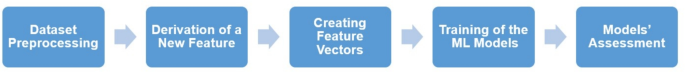
In this section, we implement and test several ML-based models using the VeReMi dataset. The implementation process has been accomplished in five phases, as summarized in Fig. 1. First, the dataset was prepared to be compatible with ML training. A new derived feature based on the received message’s RSSI was introduced in the next phase. Then, the new feature is added to a set of commonly used features to create three feature set combinations. In the fourth phase, four ML algorithms were trained using the three feature sets. Finally, the efficiency of all models was evaluated to select the best model.

Dataset preprocessing

The VeReMi dataset comprises 19 features distributed between the message logs for every simulated node and a file that specifies the actual behavior of each simulated node (ground truth file). The message logs include the reception time, the claimed location and speed of the sender in the X, Y, and Z directions, the claimed sending time, the ID of the sender and the message, and the RSSI. Conversely, the other features added by the ground truth file are the sender’s true location and speed prior to manipulation, the actual transmission time, and the attack type.

Additionally, the dataset includes five simulation repetitions, each with a set of separate sub-datasets for each attack type, at three different traffic and attack densities. These repetitions, produced using varying random seeds, offer multiple simulation runs and message logs.

Thus, before model training, several preprocessing steps were applied. First, all message logs were consolidated into a single dataset representing the complete simulation. Empty or unused features were removed, and each message was associated with its corresponding ground truth information. In addition, a merged dataset was constructed by combining all attack variants into a binary classification setting, consisting of one class representing malicious messages and another representing legitimate messages.

The categorical labels corresponding to attack types were encoded using integer label encoding prior to model training. All remaining features are continuous numerical values derived directly from the BSMs or computed during preprocessing; therefore, feature normalization or scaling was not applied.

Proposed feature

In this phase, a new feature that relies on the RSSI of the received BSM is derived to enhance the detection of position falsification attacks. RSSI represents the calculated power level of a received radio signal, expressed in decibels relative to a milliwatt (dBm). It is a key metric in wireless communication systems that can be used to measure the quality of a signal and estimate the distance between a transmitter and a receiver⁴³. However, directly using the RSSI for location estimation can lead to inaccurate outcomes due to external factors like signal fading and environmental obstacles⁴⁴.

Rather than using RSSI as an independent feature or directly calculating the sender-receiver distance, the proposed feature correlates RSSI values with their confidence intervals at a given distance range. This concept is inspired by the work of³⁰, which introduced RSSI-based plausibility checks to detect location spoofing using predefined RSSI confidence ranges. However, their approach did not incorporate ML techniques or other BSM features, relying solely on predefined thresholds. Additionally, their method employed a fixed confidence level of 99.7% in all calculations. In contrast, the proposed method assigns a location reliability score to each message using three different confidence levels, reflecting the degree of trust in the sender’s claimed location. This score is not a standalone classification mechanism but rather an enhancement that, when integrated with other key features, strengthens the detection of position spoofing attacks through ML techniques.

Initially, the RSSI confidence intervals were calculated in each distance range. To achieve this, a dataset version was created that contained only legitimate messages. Then, the sender-receiver distance (\(d_s\)) for each message was computed using the Euclidean distance. The Euclidean distance can be calculated using the following formula:

where \(x_s\) and \(y_s\) are the sender coordinates and \(x_r\) and \(y_r\) are the receiver coordinates, in the X and Y directions⁴⁵. Then, the dataset was segmented into several segments using the computed distance. For each segment, i.e., distance range, the RSSI distribution was used to calculate the RSSI confidence intervals based on its mean and variance at that distance range.

The confidence interval of sample statistics reflects the values within which the valid population parameter is expected to lie, given a specified confidence level or probability. The probability assigned to this range is the confidence level, while the higher and lower values are referred to as confidence boundaries. The following equation can identify these boundaries:

where B is the upper or lower boundary, m is the sample’s mean, z is a value that depends on the specified confidence level, sd is the sample’s standard deviation, and n is the sample size⁴⁶. The confidence intervals vary according to the chosen confidence level, as a higher confidence level results in a broader range.

Thus, instead of using a single confidence level, the RSSI confidence intervals for each distance segment were calculated at 90%, 95%, and 99% confidence levels. Figure 2 illustrates the RSSI confidence boundaries when the sender-receiver Euclidean distance ranges from 2 to 4 units. Then, all results were stored in a dictionary that associates each distance range with its respective RSSI confidence intervals. Table 3 provides a sample of the data within the created dictionary. Later, this precomputed dictionary can be published to vehicles via RSUs or by equipping cars with predefined dictionaries, to enable distributed deployment of the detection model.

The location of a received message can be classified as spoofed or not by checking whether the RSSI value falls within the confidence intervals associated with the claimed distance. To measure the effectiveness of this classification approach, the true positives, true negatives, false positives, and false negatives were calculated for the classification of BCM using confidence intervals at the three confidence levels. The performance results, as shown in Table 4, indicate that using a 90% confidence level yields the lowest precision and the highest recall, due to an increase in the count of false positives and a reduction in the count of false negatives. On the other hand, the 99% confidence level, which uses a wider interval, results in the highest precision and the lowest recall due to the reduced number of false positives and the increased number of false negatives.

Building on these findings, a new feature called “RSSIConf” was developed to break the dependency on a single confidence interval. In this feature, the RSSI value in each BSM is compared to the confidence intervals at the three distinct levels corresponding to the stated sender-receiver distance. The RSSIConf feature is then assigned a value of 3 if the RSSI is within the 90% confidence interval, 2 for the 95% interval, and 1 for the 99% interval. If the RSSI does not fall within any of these intervals, RSSIConf is set to 0, suggesting a higher risk of data fabrication. This feature derivation process was repeated for all dataset rows to add the new feature to the training dataset, as explained in Fig. 3.

It is important to note that the computationally intensive task of generating the RSSI confidence intervals and constructing the distance-to-RSSI dictionary is performed offline. Once constructed, the dictionary can be stored locally or distributed to vehicles via roadside units. During online operation, the RSSIConf feature calculation requires only a simple dictionary lookup to retrieve the corresponding confidence intervals for the claimed sender–receiver distance, followed by a small number of comparison operations. As a result, the runtime complexity of RSSIConf computation is constant time, introducing minimal computational overhead and enabling efficient real-time deployment in VANET environments.

Creating feature vectors

In this phase, we combine the newly derived feature with commonly selected and derived features to create several feature sets. This approach aims to enhance the model’s reliability, as using all of the existing BSM features to implement ML-based MDSs without incorporating feature engineering techniques can lead to potential bias and inflated results that significantly drop when models are assessed using simulations distinct from those employed during development⁴⁷. Pearson’s correlation coefficient (PCC) technique was employed to identify the most effective BSM features for attack classification. The PCC quantifies the degree of similarity and the strength of the relationship between two variables, reflecting their level of dependence⁴⁸. By performing correlation analysis on the features, it becomes possible to detect redundancies within the dataset. Additionally, examining the relationship between features and classification labels helps identify which features have a significant influence on the classification process⁴⁹. The analysis results suggest a strong correlation between the sender’s location and speed along the X and Y coordinates, as well as the identification of location manipulation attacks.

PCC was employed in this analysis instead of other ranking-based methods, such as Spearman’s rank correlation (SPC), as PCC is widely used in VANET feature selection studies for identifying redundant and highly dependent features prior to machine learning training. The objective of the feature selection stage in this work is not only to examine the relationships between features and the classification labels, but also to reduce feature redundancy among the selected attributes. Since the considered BSM features represent continuous-valued physical measurements, PCC provides an effective and sufficient measure for detecting linear dependencies and redundancy among such features.

Finally, the selected feature set was enhanced by integrating derived features that have shown strong performance in previous studies. The survey identified two frequently utilized derived features in high-performing models. These features include the variance in the sender’s reported location between consecutive BSMs and the sender-receiver distance. Additionally, other differential features were considered, such as variations in the sender’s speed and transmission time between consecutive BSMs, as well as the sender’s most recent broadcast position and speed. These features were organized into three distinct feature vectors (FV1, FV2, and FV3), as outlined in Table 5, where features marked with the symbol “*” denote the features included in the corresponding feature vector and were computed prior to model training.

Training the models

In the training phase, multiple BCS and BCM classification models were developed by training RF, KNN, XGB, and MLP ML algorithms using the three created feature vectors. RF and KNN were chosen because they are often used in high-performing models, while XGB was employed because of its high performance and robustness to overfitting⁵⁰. In addition, the MLP algorithm was chosen to experiment with a simple neural network architecture because of its outstanding efficiency in BCM classification, as presented by Kim et al.⁴².

All experiments were conducted on a Windows-based system using Python 3.7.6 within the Jupyter Notebook environment provided as part of the Anaconda Distribution (Anaconda3-2020.02) (https://www.anaconda.com/download). The ML models were implemented using the scikit-learn and XGBoost Python libraries. For each algorithm, key hyperparameters were selected based on a trade-off between detection performance and computational efficiency, with particular consideration for real-time VANET deployment constraints. For instance, since RF and XGB are ensemble learning techniques, it is necessary to initialize the count of decision trees built during training. This number is a critical parameter that influences both generalization performance and computational cost. In this study, the number of trees was set to 50. Preliminary experiments showed that increasing the number of trees beyond this value resulted in negligible performance improvements while substantially increasing training and inference time. Consequently, 50 trees were selected as a balanced configuration that provides stable performance without unnecessary computational overhead.

The KNN classifier assigns class labels based on the majority class of the training set’s nearest neighbors, where ‘k’ is the count of neighbors used in the classification. The value of ‘k’ was set to 3, as using small values of ‘k’ reduces the number of distance calculations and sorting operations required during inference, which is desirable in time-sensitive VANET applications. Initial testing indicated that larger k values increased computational cost and slightly smoothed decision boundaries without yielding consistent performance gains.

For the MLP classifier, the network architecture was adopted from the configuration reported in⁴², which demonstrated strong performance for similar misbehavior detection tasks. The architecture consists of three hidden layers, each with eight neurons, using “ReLU,” “ReLU,” and “Sigmoid” activation functions, respectively. All remaining hyperparameters for the evaluated models were kept at their default values to avoid unnecessary complexity.

Overall, initial experimental evaluations indicated that moderate variations around the selected hyperparameter values did not lead to significant changes in classification performance, whereas larger deviations mainly increased computational cost without improving detection accuracy.

Models’ assessment

In the assessment phase, the performance of all pre-trained schemes was used to select the model with the highest performance. Four Key Performance Indicators (KPIs) were employed to assess the models’ efficiency. The first KPI is accuracy, which measures the model’s ability to identify positive and negative inputs. Thus, accuracy increases when true positive and true negative rates are higher. However, focusing on accuracy may be insufficient for assessing MDS performance, particularly with imbalanced datasets⁵¹. Precision, the second KPI used, is the proportion of correctly identified positive samples to the total number of predicted positive samples. The third measure, recall, assesses the system’s ability to determine actual positive samples accurately. The last KPI is the F1-score, which provides a balanced statistic that considers both false positives and negatives³⁸.

The models were tested using a randomly chosen 30% subset of each dataset. Tables 6, 7, 8, 9, 10 and 11 present the performance results obtained for all tested models. The outcomes show that the RF model achieved 100% measures for the CP attack detection when employing any of the three feature vectors (FV1, FV2, or FV3). The XGB model achieved the same perfect performance using FV1 and a near-perfect performance using FV2 and FV3. In the COP attack, both RF and XGB models achieved over 99.9% performance employing any of the three feature vectors. However, the XGB models showed a very slight enhancement over the RF models.

For the RP attack, both RF and XGB models achieved over 99.9% performance employing FV2 and FV3. However, the RF model with FV2 (RF-FV2) outperformed the others, achieving the best results among all tested models with a very slight increase in recall percentage. Furthermore, in detecting ROP and ES attacks, the RF-FV3 models outperformed other models. For example, in the ROP attack, the RF-FV3 model achieved a detection accuracy of 99.72% and an F1-score of 99.67%. Similarly, the achieved accuracy and F1-score were 99.9% and 99.88% in the ES attack detection. When used for BCM classification, the RF-FV3 model achieved the highest performance, with 99.86% accuracy and a 99.85% F1-score.

The research findings show that although the XGB-FV2 and XGB-FV3 models had almost similar performance to the RF-FV2 and RF-FV3 models in detecting CP, COP, and RP attacks, they were less efficient in ROP, ES, and BCM classification. These results also indicate that employing RF with either FV2 or FV3 is almost equally successful at identifying the five attack types, including BCM categorization, with only a slight performance increase provided by RF-FV3 in ROP, ES, and BCM classification, which does not exceed 0.02%. Thus, both RF-FV2 and RF-FV3 can be considered the top models among the trained models. This observation is further supported by the confusion matrices obtained for the RF-FV2 and RF-FV3 models in the BCM classification. As illustrated in Figures 4 and 5, both models achieve very high true positive and true negative rates, with only marginal misclassification between benign and attack classes. Confusion matrix analysis is presented for FV2 and FV3 only, as FV1 consistently exhibited lower performance across all evaluated metrics and attack types; therefore, its confusion matrix was omitted to maintain focus on the most competitive feature sets.

The processing time of a pre-trained model, measured from message reception to output classification, was included in the performance comparison of the models. This metric provides an estimate of the computational efficiency of the models during deployment and is calculated by dividing the total testing time by the number of samples processed. Figure 6 presents a comparative analysis of the average classification time for the RF-FV2 and RF-FV3 models across individual attack types as well as the BCM scenario.

For CP and RP attacks, RF-FV3 exhibits a slightly higher classification time than RF-FV2, which can be attributed to the additional feature processing introduced by the expanded feature set. In contrast, for COP, ROP, and ES attacks, both models demonstrate nearly identical execution times, indicating that the added features in FV3 do not noticeably impact runtime for these scenarios. In the BCM case, the execution-time difference becomes more pronounced, with RF-FV3 performing up to 25% slower than RF-FV2. This behavior can be explained by the fact that the BCM dataset encompasses a larger and more diverse set of samples, which increases the number of feature evaluations required per classification. Overall, these results indicate that RF-FV2 incurs lower computational cost.

In real VANET environments, multiple position falsification attacks can occur at the same time, so deploying multiple specialized detection models is a realistic issue in terms of feasibility. While training individual models for every attack might provide worthwhile insights, deploying multiple models simultaneously would incur greater computational cost and undermine efficiency in real-time applications. Therefore, the primary objective of training individual models within this study was to facilitate a comparison of how the selected sets of features and ML algorithms performed on various attack types, which is a commonly used methodology in related literature.

Based on the above evaluation, the RF-FV2 model was selected as the primary detection model because it provides a favorable trade-off between detection accuracy and computational efficiency, as reflected in its consistently strong performance across all evaluated attack types and its lower inference latency compared to alternative models. In addition, RF effectively handles heterogeneous and correlated features with limited sensitivity to parameter tuning, which contributes to stable generalization performance and makes it suitable for real-time deployment in dynamic VANET environments⁵². Moreover, RF-FV2 was trained and tested under the BCM classification scenario, which incorporates all five attack categories, and achieved high detection performance, making it a more representative and reliable choice for deployment in realistic VANET settings.