
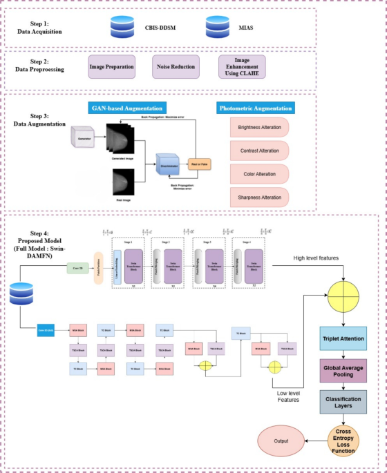
This study introduces Swin-DAMFN, a novel dual-branch deep learning architecture for breast cancer classification from mammograms, designed to exploit both global contextual information and fine-grained local features. As illustrated in Fig. 1, the overall framework begins with dataset preparation, followed by preprocessing and augmentation strategies to enhance data quality and balance class distribution. The processed images are then fed into the proposed dual-branch model for feature extraction and classification. The network architecture of Swin-DAMFN, depicted in Fig. 2, consists of two complementary branches. The first branch employs a Swin Transformer, which captures long-range global dependencies across breast tissue through its hierarchical structure and shifted-window attention mechanism. The second branch, the Dual-Attention Multi-scale Fusion Network (DAMFN), is a CNN-based pathway designed to extract discriminative local patterns such as microcalcifications and mass margins. DAMFN integrates three specialized blocks: (i) Multi-Separable Attention (MSA), (ii) Tri-Shuffle Convolution Attention (TSCA), and (iii) a Traditional Convolution (TC) block, each operating at multiple receptive fields to capture fine-grained multi-scale information.
Features from both branches are fused using depth-wise concatenation, refined through a Triplet Attention (TA) block, and pooled via Global Average Pooling (GAP). The final classification is performed by fully connected layers with cross-entropy as the loss function. This architecture ensures that both global and local information contribute effectively to the final decision, thereby enhancing the robustness and clinical reliability of the model.

Overview of the proposed Swin-DAMFN architecture for breast cancer classification.

Proposed Swin-DAMFN architecture for breast cancer classification.
Dataset description
This study eutilizes two publicly available benchmark datasets, the Curated Breast Imaging Subset of DDSM (CBIS-DDSM) and the Mammographic Image Analysis Society (MIAS) database, to evaluate the performance of the proposed model Mammography is a critical tool for the early detection of breast cancer, primarily through the identification of masses and calcifications in X-ray images52. To guarantee that no patient appears in more than one split (training/validation/test), the datasets were divided at the patient level for CBIS-DDSM using the supplied patient IDs. Image-wise splitting was used with rigorous manual verification for the MIAS dataset, which lacks specific patient identification, in order to prevent any implied overlap of the same breast or laterality/view.
CBIS-DDSM dataset
The CBIS-DDSM is an updated and standardized version of the original Digital Database for Screening Mammography (DDSM)53. This curated dataset offers significant improvements, including images in the standardized DICOM format and a restructured, more accessible metadata organization. It comprises 1,459 mammograms annotated across four diagnostic categories: Benign Calcification (398 images), Benign Mass (417 images), Malignant Calcification (300 images), and Malignant Mass (344 images). All mammograms were preprocessed by resizing them to a uniform resolution of \(224 \times 224\) pixels.
MIAS dataset
The MIAS database was used to assess the suggested model’s robustness and generalizability54. This dataset, which was assembled by a collection of UK research groups, includes 322 mammograms divided into three classes: benign (63 images), malignant (52 images), and normal (207 images).
A summary of the key characteristics of both datasets is provided in Table 2. The MIAS dataset classification task is carried out as a three-class issue (Benign, Malignant, and Normal), with the Normal class being handled as a separate category. As previously mentioned, the CBIS-DDSM dataset is classified into four classes. The model employs categorical cross-entropy loss in both scenarios, and assessment metrics (such as sensitivity) are macro-averaged over all classes. In MIAS, the Normal class is treated in the same way as other classes during feature extraction and fusion, which take place before the classification head.
Data preprocessing
Accurate identification of breast lesions within the surrounding tissue presents a significant diagnostic challenge, with a non-negligible potential for misdiagnosis55. These lesions are often characterized geometrically by features such as origin, size, and perimeter, and typically appear brighter than the adjacent breast tissue56. Radiologists often compare mammograms of the same breast taken over time to monitor the progression of lesions. This temporal analysis relies on identifying stable control points (e.g., tissue junctions, duct intersections, vascular features) and calculating correlations between these points across sequential images. Adapting deep learning models to this complex environment is a critical challenge in medical image analysis. Preprocessing is a crucial step in enhancing the signal-to-noise ratio, thereby improving the distinction between normal anatomical structures and pathological features. To mitigate the risk of overfitting and improve model generalization, a series of preprocessing steps, including noise removal, image enhancement, scaling, and cropping, is applied prior to training.
In this paper, we employ a combination of techniques to improve mammogram readability and feature prominence. This includes mean and median filtering for noise reduction, morphological operations to refine structures, and Contrast Limited Adaptive Histogram Equalization (CLAHE) to enhance local contrast without amplifying noise.
Image preparation
The acquisition of a large, high-quality dataset of mammography images presents significant practical challenges. Raw mammograms contain sensitive patient information, inherent noise, and variabilities in lighting conditions, all of which can contribute to a higher rate of false positives in automated analysis. To mitigate these issues while preserving critical information, images are converted to a grayscale format. The inherent limitations of mammography, combined with a scarcity of available images, pose a major obstacle to training accurate deep learning models. Data scarcity often leads to overfitting, in which models perform well on training data but fail to generalize to new examples. Furthermore, annotating breast images for supervised algorithm training is labor-intensive and costly57. To prepare the images for analysis, morphological operations, specifically opening and closing, are applied to remove identifying labels and annotation tags. These operations are based on the fundamental processes of erosion and dilation, which reduce and expand the sizes of structures within an image, respectively.
The erosion of a set E by a structuring element S is defined as the set of all points p for which S translated by p is entirely contained within E:
$$\begin{aligned} E \ominus S = \{ p \mid (S)_{p} \subseteq E \} \end{aligned}$$
(1)
The dilation of E by S is defined as the set of all points p for which the reflected structuring element \(\hat{S}\) translated by p has a non-empty intersection with E:
$$\begin{aligned} E \oplus S = \{ p \mid (\hat{S})_{p} \cap E \ne \emptyset \} \end{aligned}$$
(2)
Opening and closing stem from these fundamental operations. An opening is defined as erosion followed by dilation. It is used to remove small, bright artifacts and break thin connections. Closing is defined as dilation followed by erosion. Closing is used to remove small, dark holes and fuse narrow breaks.
$$\begin{aligned} \text {Opening:} \quad&E \circ S = (E \ominus S) \oplus S \end{aligned}$$
(3)
$$\begin{aligned} \text {Closing:} \quad&E \cdot S = (E \oplus S) \ominus S \end{aligned}$$
(4)
In this work, these morphological operations, defined by Eqs. 3 and 4 are employed to effectively eradicate labeling and annotation markers from the mammography images while preserving the essential features of the underlying breast tissue. Furthermore, let I be the input image with dimensions \(H \times W \times C\) (height, width, channels). After grayscale conversion, \(C = 1\), and the image is normalized to [0,1] range using \(I_{norm} = (I – \min (I)) / (\max (I) – \min (I))\).
Image noise reduction
Following acquisition, mammography images undergo processing to eliminate various forms of noise that can degrade image quality and hinder accurate analysis. Common noise types in these images include Gaussian, salt-and-pepper, speckle, and Poisson noise. To address this, we employ an adaptive median filtering approach, which processes the noisy input image \(I_n\) to produce a denoised output image \(I_{nf}\). The adaptive median filter is particularly effective at suppressing impulse noises, such as salt-and-pepper noise, while preserving edges and details. The algorithm operates as follows:
-
1.
Initialization: For each pixel, a sliding window of size \(CR_w\) is defined. The minimum and maximum pixel intensities within this window are identified as \(MinP_w\) and \(MaxP_w\), respectively. The median value within the window is calculated as \(Med_w\). The parameter \(MaxP_w\) represents the maximum allowable window size for the adaptive process.
-
2.
Impulse detection: The condition \(MinP_w< Med_w < MaxP_w\) is evaluated. If this condition is satisfied, \(Med_w\) is not considered an impulse noise pixel, and the algorithm proceeds to the next step. If not, the window size \(CR_w\) is increased. Step 1 is repeated until either the median value is no longer an impulse or the window reaches its maximum allowed size (\(CR_w = MaxP_w\)). If the maximum size is reached, the median value is assigned as the filtered output for the pixel.
-
3.
Pixel replacement: If the median was deemed not to be an impulse in Step 2, the algorithm then checks the original pixel value \(I_n\). If \(MinP_w< I_n < MaxP_w\), the pixel is considered uncorrupted, and its value remains unchanged in the filtered image (\(I_{nf} = I_n\)). However, if \(I_n\) equals either \(MinP_w\) or \(MaxP_w\), it is classified as corrupted. In this case, it is replaced by the median value obtained in Step 2 (\(I_{nf} = Med_w\)).
Mathematically, for a pixel at position (i, j), the adaptive median \(Med_w(i,j) = \text {median} \{ I_n(k,l) \mid (k,l) \in W \}\), where W is the window centered at (i, j). The window size \(CR_w\) starts at 3×3 and increases by 2 until \(MaxP_w = 7×7\) or the condition is met. This adaptive process ensures effective noise reduction while minimizing the blurring of fine details and edges, which are crucial for accurate medical image analysis.
Image enhancement using CLAHE
A widely adopted method in medical image processing for enhancing local contrast is contrast-limited adaptive histogram equalization (CLAHE). It functions by partitioning the input image into smaller, non-overlapping regions, known as tiles. Within each tile, a histogram of pixel intensities is calculated and adjusted using a predefined clip limit, which prevents the over-enhancement of noise. The clipped pixels are then evenly redistributed across all histogram bins, ensuring contrast enhancement while maintaining visual consistency and suppressing artifacts58,59. The total number of tiles, represented by T, is computed by the following expression:
$$\begin{aligned} T = \frac{N \times N}{n \times n} \end{aligned}$$
(5)
where N is the total image dimension and n is the size of each tile.
To enhance visual quality effectively, the algorithm applies a Normalized Contrast Limit (NCL), while the average number of pixels in the image (\(NAV_G\)) is given by:
$$\begin{aligned} NAV_G = \frac{N_x \times N_y}{N_g} \end{aligned}$$
(6)
Here, \(N_g\) represents the number of grayscale levels, and \(N_x\) and \(N_y\) correspond to the pixel dimensions along the x and y axes, respectively.
The mean number of clipped pixels per bin, \(N_{cp}\), is derived using:
$$\begin{aligned} N_{cp} = \frac{\sum CL}{N_g} \end{aligned}$$
(7)
where \(\sum CL\) is the total number of pixels exceeding the clip limit.
Any remaining pixels, which are not distributed by this process, are uniformly spread across all grayscale levels using:
$$\begin{aligned} R = \frac{N_g}{N_r} \end{aligned}$$
(8)
where \(N_r\) denotes the number of remaining unallocated pixels. For a tile histogram h(b) with bin \(b = 0, \dots , L-1\) (where \(L = 256\) for 8-bit grayscale), the clip limit \(clip = \alpha \cdot (NAV_G / L)\), where \(\alpha\) is the clip factor (typically 0.01 to 0.03). The cumulative distribution function (CDF) for mapping is \(CDF(b) = \sum _{k=0}^b h'(k) / \sum h'(k)\), where \(h’\) is the clipped histogram.
Data augmentation
Medical imaging datasets for breast cancer detection are often limited in size and suffer from class imbalance, which can negatively impact the performance and generalization ability of deep learning models. In particular, the MIAS dataset suffers from a small number of samples, while the CBIS-DDSM dataset exhibits class imbalance with malignant lesions being relatively underrepresented. These challenges increase the risk of overfitting and hinder the ability of deep learning models to generalize to unseen data. To overcome these challenges, we adopted a hybrid augmentation strategy that integrates Generative Adversarial Networks (GANs)60 with photometric augmentation techniques. The GAN-based augmentation was employed to generate realistic mammogram samples, particularly for minority classes, thereby addressing the imbalance problem. In parallel, photometric augmentation was applied to enhance data diversity by altering brightness, contrast, color, and sharpness levels of the original images. The combination of these two approaches not only increased the dataset size but also enriched its quality and variability, resulting in a more balanced and comprehensive dataset for training. The overall distribution of the datasets before and after augmentation is summarized in Table 3.
GAN-based augmentation
Class imbalance and the lack of annotated mammograms were addressed using GANs. The Generator and Discriminator neural networks make up a GAN framework. These networks undergo adversarial training. The generator learns to create realistic images and simulate the distribution of actual mammograms. The discriminator, meanwhile, attempts to distinguish between generated and actual images. The generator may gradually produce realistic, high-quality mammograms that capture fine-grained diagnostic patterns, such as masses and microcalcifications, as well as global tissue features, thanks to this adversarial training process. When the discriminator can no longer consistently distinguish between real and synthetic samples (i.e., when it converges to about 50% accuracy), the GAN training is said to be stable. The GAN architecture overview is shown in Fig. 3.

The objective function of the GAN is defined using Eq. (9):
$$\begin{aligned} \chi (G, D) = \min _{G} \max _{D} \Big \{ \mathbb {E}_{x \sim p_{\text {data}}(x)}[\log D(x)] + \mathbb {E}_{z \sim p_{z}(z)}[\log (1 – D(G(z)))] \Big \}, \end{aligned}$$
(9)
where x represents a real mammogram, z is a random noise vector, G(z) is the generated synthetic mammogram, D(x) and D(G(z)) denote the Discriminator outputs for real and synthetic images, respectively, and \(p_{\text {data}}\) and \(p_{z}\) represent the real data and noise distributions.
In our study, GAN-based augmentation is applied differently to the two datasets:
-
MIAS: Due to the small dataset size, GANs are used to significantly expand the number of training samples, particularly for the minority malignant class, thus reducing overfitting and improving model generalization.
-
CBIS-DDSM: GANs are selectively applied to balance the class distribution by synthesizing malignant cases, thereby reducing bias toward benign classes. This ensures that the classifier does not become skewed by class imbalance.
In this study, GAN augmentation was particularly effective for minority classes such as malignant lesions in the MIAS dataset and malignant calcifications in CBIS-DDSM. By generating realistic mammograms for these underrepresented categories, GANs significantly improved the class balance and enhanced the diversity of the training set.
conditional deep convolutional GAN (cDCGAN)
To create realistic mammograms for minority classes, a conditional Deep Convolutional GAN (cDCGAN)61 was used just on the training split. Five transposed convolutional layers with batch normalization and ReLU activations make up the generator, while five convolutional layers with LeakyReLU activations make up the discriminator. For 200 epochs (CBIS-DDSM) and 300 epochs (MIAS), training employed the Adam optimizer (learning rate \(2\times 10^{-4}\), \(\beta _1 = 0.5\), \(\beta _2 = 0.999\)) with mini-batch size 16. In order to maintain anatomical structures, the objective mixed an L1 reconstruction term with a non-saturating adversarial loss. The generator uses transposed convolutions (kernels 4×4, stride 2) with batch normalization and ReLU, while the discriminator uses convolutions (kernels 4×4, stride 2) with LeakyReLU (slope 0.2). The loss is non-saturating adversarial + L1 reconstruction (?=100). Early stopping is applied if discriminator accuracy stabilizes around 50% for 10 epochs. The augmented dataset sizes displayed in Table 3 were obtained by generating three to five synthetic photos for each real minority-class sample. A balanced 50:50 combination of real and synthetic images was present in each mini-batch during training.
The realism of synthetic mammograms was quantitatively evaluated using the Fréchet Inception Distance (FID) as shown in Eq. (10):
$$\begin{aligned} d^2\big ((m, C), (m_w, C_w)\big ) = \Vert m – m_w\Vert _2^2 + \textrm{Tr}\!\left( C + C_w – 2\left( CC_w\right) ^{1/2}\right) \end{aligned}$$
(10)
where m, C and \(m_w, C_w\) are the mean and covariance of feature embeddings (pretrained Inception-v3) of real and synthetic images, respectively. Lower values indicate higher similarity. Our model achieved an average FID of 18.7, indicating strong visual realism.
Qualitative inspection of generated samples confirmed high fidelity and absence of obvious artifacts. Illustrative examples are shown in Fig. 4.

Illustrative examples of real (left column) and synthetic (right columns) high-density mammograms generated using CycleGAN-based models (adapted from published literature on mammography synthesis). (A) CC view, (B) MLO view. Green boxes highlight regions of interest (e.g., microcalcifications).
While GAN-based augmentation significantly reduces data imbalance and enhances model generalization, it may also cause a shift in the distribution between the real and synthetic mammography domains. To mitigate this risk, the training phase utilized only synthetic samples, and the testing and validation subsets did not contain any actual data. However, we recognize that a classifier trained on a combination of actual and synthetic data would not be able to generalize to images that are exclusively clinical. To overcome this constraint, future research will utilize adversarial realignment techniques and domain adaptation on actual multi-institutional datasets.
Photometric augmentation
The brightness factor in [0.8, 1.2], contrast in [0.8, 1.2], and sharpness in [0.8, 1.2] are examples of specific transformations that are applied at random with a probability of 0.5. In addition to GAN-based augmentation, photometric augmentation techniques were employed to further enrich the dataset’s diversity. Unlike generative approaches, photometric augmentation modifies the pixel intensity distributions of existing images, producing multiple qualitative variations while preserving the original anatomical structures. Four types of transformations were considered:
-
Brightness alteration: Adjusts the illumination of the image. Factors greater than 1 increase brightness, while values less than 1 decrease it. A factor of 0 results in a completely black image.
-
Contrast alteration: Modifies the ratio between light and dark regions. Higher factors amplify differences between bright and dark regions, while lower values reduce contrast.
-
Color alteration: Alters the intensity of RGB channels. A factor greater than 1 enhances color saturation, values between 0 and 1 desaturate the image, and a factor of 0 converts the image to grayscale.
-
Sharpness alteration: Enhances or smoothens edges. Larger factors sharpen borders and edges, whereas smaller values produce a blurred effect.
Although both CBIS-DDSM and MIAS datasets are widely used in breast cancer research, they suffer from severe class imbalance, where malignant cases are notably underrepresented compared to benign and normal samples. This imbalance negatively impacts classification performance, particularly in terms of sensitivity to malignant tumors. To mitigate this issue, GANs were primarily utilized to oversample minority classes by generating realistic synthetic mammograms, thereby achieving a more balanced class distribution. Additionally, photometric augmentation techniques, including adjustments to brightness, contrast, color, and sharpness, were applied to enhance data diversity and improve generalization. These complementary strategies not only expanded the dataset size but also reduced bias between classes, resulting in a nearly balanced distribution across all categories. Table 3 presents the final dataset distribution after augmentation.
Proposed Swin-DAMFN architecture
Swin Transformer
The Swin Transformer branch captures global context and long-range dependencies in mammograms, which is essential for detecting the diffuse patterns and structural asymmetries indicative of breast cancer. As illustrated in Fig. 5, its hierarchical architecture employs a shifted window mechanism to achieve efficient multi-scale feature learning with computational complexity that scales linearly with input size62. The process initiates with patch partitioning, where the input mammogram (of dimensions \(H \times W \times 3\)) is divided into non-overlapping \(4 \times 4\) patches. Each patch is subsequently embedded into a C-dimensional vector through a linear layer. These embedded tokens are then hierarchically refined by passing through four sequential stages of Swin Transformer blocks.
The input mammogram has dimensions \(224 \times 224 \times 3\). After patch partitioning into \(4 \times 4\) patches and linear embedding to \(C=96\) dimensions, the feature map is \(56 \times 56 \times 96\). Subsequent patch merging reduces resolutions to \(28 \times 28 \times 192\) (Stage 2), \(14 \times 14 \times 384\) (Stage 3), and \(7 \times 7 \times 768\) (Stage 4).
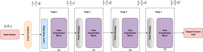
The architecture of the Swin Transformer.
A key innovation is the Shifted Window-based Self-Attention (SW-MSA) mechanism. Unlike standard Vision Transformers that compute self-attention globally, the Swin Transformer limits computation to non-overlapping local windows. Between consecutive blocks, the window partitioning scheme is shifted, facilitating cross-window communication and significantly enhancing modeling capability without a quadratic increase in computational cost. The complexity for an image with \(h \times w\) patches is given by:
$$\begin{aligned} \Omega (\text {MSA})&= 4hwC^2 + 2(hw)^2C, \end{aligned}$$
(11)
$$\begin{aligned} \Omega (\text {W-MSA})&= 4hwC^2 + 2M^2 hwC, \end{aligned}$$
(12)
where M is the window size and C is the feature dimension.
Each stage reduces the spatial resolution while increasing the feature dimensionality through a Patch Merging layer, which concatenates features from groups of \(2 \times 2\) adjacent patches and applies a linear layer. This results in feature maps at resolutions of \(\frac{H}{4} \times \frac{W}{4}\), \(\frac{H}{8} \times \frac{W}{8}\), \(\frac{H}{16} \times \frac{W}{16}\), and \(\frac{H}{32} \times \frac{W}{32}\) across the four stages, respectively.
The Swin transformer blocks utilize W-MSA and SW-MSA modules consecutively to extract features and spatial correlations from the input data. Figure 6 depicts the connection between two successive Swin transformer blocks.
A Swin Transformer block is formulated as:
$$\begin{aligned} \hat{\textbf{z}}^l&= \text {W-MSA}(\text {LN}(\textbf{z}^{l-1})) + \textbf{z}^{l-1}, \end{aligned}$$
(13)
$$\begin{aligned} \textbf{z}^l&= \text {MLP}(\text {LN}(\hat{\textbf{z}}^l)) + \hat{\textbf{z}}^l, \end{aligned}$$
(14)
$$\begin{aligned} \hat{\textbf{z}}^{l+1}&= \text {SW-MSA}(\text {LN}(\textbf{z}^l)) + \textbf{z}^l, \end{aligned}$$
(15)
$$\begin{aligned} \textbf{z}^{l+1}&= \text {MLP}(\text {LN}(\hat{\textbf{z}}^{l+1})) + \hat{\textbf{z}}^{l+1}, \end{aligned}$$
(16)
where \(\hat{\textbf{z}}^l\) and \(\textbf{z}^l\) denote the outputs of the (S)W-MSA module and the MLP module for block l, respectively. LayerNorm (LN) and residual connections are applied before each module to stabilize the training process.
The output from the final stage, a rich set of 96 global features, is subsequently forwarded to the fufor integratione integrated with the local features extracted by the DAMFN track.

Interconnection between two consecutive Swin Transformer blocks.
Dual-Attention Multi-scale Fusion Network (DAMFN) track
The Dual-Attention Multi-scale Fusion Network (DAMFN) track is a pivotal component of our proposed architecture, working in synergy with the Swin Transformer pathway. As illustrated in Fig. 7, the DAMFN track is specifically engineered to process input mammography images at their original resolution of \(224 \times 224 \times 3\), ensuring no loss of critical, fine-grained details essential for accurate diagnosis.
This branch is dedicated to extracting and refining hierarchical, multi-scale features from the input data. Its core objective is to capture low-level spatial dependencies and intricate local patterns–such as tissue texture, micro-calcifications, and mass margins–that are paramount for distinguishing malignant from benign lesions. The DAMFN incorporates dedicated attention mechanisms within its blocks to dynamically highlight these clinically relevant regions while suppressing irrelevant background information, ensuring the model focuses its computational resources on the most discriminative features.
The DAMF is composed of three fundamental blocks: the Multi-Scale Attention (MSA) block, the Two-Step Channel Attention (TSCA) block, and the Traditional Convolutional (TC) block. In the final stage of the track, the MSA and TSCA blocks operate in parallel. Their outputs are concatenated and subsequently processed by a final TC block. This design enhances the network’s adaptability and efficacy in capturing a diverse spectrum of features across multiple scales and spatial contexts, significantly contributing to the model’s robustness. The cumulative output of this track is a rich, high-dimensional feature map that is seamlessly fused with the global, contextual features extracted by the Swin Transformer track, providing a comprehensive feature set for the final classification stage.
The input is \(224 \times 224 \times 3\). After the initial MSA block, features are \(112 \times 112 \times 32\); after TSCA, \(56 \times 56 \times 64\); after TC, \(28 \times 28 \times 128\). In the final stage, parallel MSA and TSCA outputs are concatenated to \(14 \times 14 \times 384\), then processed by TC to \(7 \times 7 \times 768\).

Multi-scale Attention (MSA) Block The MSA block is designed for efficient multi-scale feature extraction. It employs three parallel convolutional pathways: Learned Depth-wise Separable Convolutions by Group Pruning (LdsConv)63, Flexible and Separable Convolution (FSConv)64, and Depth-wise Separable Convolutions (DWSC)65. This parallel structure facilitates comprehensive feature learning at various representational levels. These advanced convolutional techniques decompose standard operations, offering a significant reduction in computational complexity and parameter count compared to traditional convolutions, without compromising representational power. The feature maps from all three pathways are concatenated and subsequently refined using a Convolutional Block Attention Module (CBAM) to amplify salient features crucial for breast cancer detection and suppress less informative noise. The structure of the MSA block is depicted in Fig. 8.
For input feature map \(F \in \mathbb {R}^{C \times H \times W}\), the LdsConv pathway is \(F_{lds} = \text {LdsConv}(F) = \text {Prune}(\text {GroupConv}(F))\), where pruning removes low-importance groups. FSConv is \(F_{fs} = \text {FSConv}(F) = \text {Depthwise}(F) + \text {Pointwise}(F)\). DWSC is \(F_{dw} = \text {DWConv}(F) + \text {Pointwise}(F)\). Concatenated features \(F_{cat} = [F_{lds}, F_{fs}, F_{dw}]\). CBAM refines as \(F’ = F_{cat} \odot \text {ChannelAtt}(F_{cat}) + F_{cat} \odot \text {SpatialAtt}(F_{cat})\), where \(\odot\) is element-wise multiplication.

Overview of the Multi-Scale Attention (MSA) architecture.
Tri-shuffle convolution attention (TSCA) block Feature maps from the MSA block are processed by the TSCA block. This block utilizes three parallel convolutional layers: group convolution, dilated convolution, and a standard convolution with kernel sizes of 3, 2, and 1, respectively. A channel shuffle operation is applied to these layers prior to the application of these layers to promote cross-group information exchange and enhance feature diversity. The group convolution reduces computational overhead by dividing the input tensor into subgroups. The incorporated dilated convolution expands the receptive field exponentially without increasing the kernel size or parameters, allowing for the capture of richer contextual information from breast tissue structures. The outputs of these parallel layers are concatenated and processed by a triplet attention mechanism, which further accentuates the most informative feature channels and spatial regions. An overview of the TSCA block is provided in Fig. 9.

Schematic representation of the Two-Scale Channel Attention (TSCA) architecture.
Traditional Convolutional (TC) Block The output from the TSCA block is further refined by the TC block. This block performs a series of standard operations to efficiently transform features and prepare them for fusion. The process initiates with batch normalization to enhance training stability, followed by a ReLU activation function to incorporate non-linearity. Feature abstraction and dimensionality reduction are achieved through a 2D max-pooling layer, while a dropout layer is applied as an effective regularization technique to mitigate overfitting. A final convolutional layer ensures the feature map has the appropriate dimensions for subsequent fusion operations.
For input \(F \in \mathbb {R}^{C \times H \times W}\), batch norm is \(F_{bn} = \frac{F – \mu }{\sqrt{\sigma ^2 + \epsilon }} \cdot \gamma + \beta\), where \(\mu , \sigma\) are mean and variance, \(\gamma , \beta\) learned parameters. ReLU: \(F_{relu} = \max (0, F_{bn})\). Max-pool: \(F_{pool} = \max (F_{relu}, k=2)\). Dropout: \(F_{drop} = F_{pool} \cdot m\), \(m \sim \text {Bernoulli}(1-p)\), \(p=0.5\). Final conv: \(F’ = \text {Conv}(F_{drop}, k=1)\).
Triplet attention (TA) block
The Triplet Attention (TA) block is a lightweight yet powerful channel and spatial attention mechanism integrated into our model. Its resource-efficient design makes it ideal for complex medical image analysis tasks without introducing significant computational overhead. The schematic of the TA block is depicted in Fig. 10. TA captures cross-dimensional dependencies between channel (C) and spatial (H, W) dimensions through three parallel branches. This approach effectively addresses the limitation of standard channel attention mechanisms by incorporating rich cross-dimensional interactions. For an input tensor \(\chi \in \mathbb {R}^{C \times H \times W}\), each branch performs a specific rotational operation followed by a Z-pooling layer and a standard convolutional layer. The Z-pool operation, which concatenates max and average pooling along the depth dimension, is defined as:
$$\begin{aligned} Z\text {-}pool(x) = [MaxPool_{0d}(x), AvgPool_{0d}(x)] \end{aligned}$$
(17)
The outputs from the three branches are then aggregated using a simple averaging operation to produce the final refined tensor:
$$\begin{aligned} y = \frac{1}{3} \left( \mathcal {R}(X_{1}^{\omega _1}) + \mathcal {R}(X_{2}^{\omega _2}) + X^{\omega _3} \right) = \frac{1}{3} (y_1 + y_2 + y_3) \end{aligned}$$
(18)
where \(\omega _1, \omega _2,\) and \(\omega _3\) represent the three cross-dimensional attention weights, \(X^{\omega _3}\) is the un-rotated weighted tensor, and \(\mathcal {R}(X_{1}^{\omega _1})\) and \(\mathcal {R}(X_{2}^{\omega _2})\) denote rotations by 90 degrees to restore the original input shape of \((C \times H \times W)\).
Branch 1 (channel-spatial H): Rotate \(\chi\) to \(H \times C \times W\), Z-pool to \(2 \times C \times W\), conv with kernel \(k=7\) to get \(\omega _1\). Branch 2 (channel-spatial W): Rotate to \(W \times C \times H\), Z-pool to \(2 \times C \times H\), conv to \(\omega _2\). Branch 3 (spatial): Z-pool to \(2 \times H \times W\), conv to \(\omega _3\). Sigmoid activation on all \(\omega\) for [0,1] weights.
In the context of breast cancer classification, the TA block enhances the model’s ability to identify and emphasize critical diagnostic patterns. It improves feature representation by highlighting salient channels and spatial regions associated with malignant findings (such as spiculated masses or micro-calcifications) while suppressing less informative features from dense breast tissue. This leads to more accurate and robust classification performance.

Overview of the triplet attention block.
Fusion model
This section describes the entire layer-by-layer architecture and fusion mechanism connecting the Swin Transformer and DAMFN branches in order to guarantee total methodological coverage and achieve complimentary feature enrichment beforehand. This fusion’s design goal is to combine the fine-grained local textures maintained by DAMFN with the high-level semantic representation collected by Swin in order to achieve complimentary feature enrichment prior to final classification. A thorough architectural breakdown of both branches is given in Table 4, which includes input/output dimensions, kernel sizes, strides, and the number of convolutional layers per stage. Direct implementation and a clear distinction between multi-scale convolutional processing and hierarchical transformer encoding are made possible by this organized presentation.
Fusion mechanism. The fusion process begins by aligning the spatial dimensions of the Swin Transformer output (\(7\times 7\times 768\)) and the DAMFN output (\(28\times 28\times 96\)). The Swin features are upsampled via bilinear interpolation to match the DAMFN resolution, ensuring pixel-wise correspondence. The two representations are then concatenated along the channel dimension, forming a composite tensor that encodes both global semantic and local structural cues. To enhance feature selectivity and suppress redundant information, a Triplet Attention module is subsequently applied across the spatial and channel axes.
Finally, a Global Average Pooling (GAP) operation aggregates the refined feature map into a compact representation, which is passed through fully connected layers for classification. The complete process is illustrated in Algorithm 1, which presents the computational flow and parameterization of each step for straightforward reimplementation.
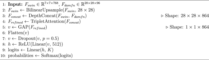
Fusion module pseudo-code
Classification head
The refined feature maps, enriched by the DAMFN and Swin Transformer tracks and processed by the Triplet Attention mechanism, are prepared for the final classification stage. To generate a fixed-length vector representation from these spatial feature maps, a GAP layer is applied. This operation summarizes each feature map by computing its average value, effectively reducing the spatial dimensions to \(1 \times 1\) while preserving the channel-wise information. This significantly reduces the number of parameters in the subsequent fully connected layers, acting as a strong regularizer to mitigate overfitting. The resulting vector is then fed into a compact classification module. This module consists of:
-
A Flatten layer to convert the pooled vector into a one-dimensional array.
-
A Dropout layer (\(p=0.5\)) for further regularization, randomly disabling a fraction of neurons during training to prevent co-adaptation and enhance generalization.
-
A fully connected (Linear) layer with ReLU activation, serving as a hidden layer for non-linear feature transformation.
-
A final fully connected (Linear) layer that projects the features into the output logits space corresponding to the number of target classes (e.g., Benign, Malignant, and optionally Normal).
For the optimization of the classification head and the entire network, the Cross-Entropy loss function (\(\mathcal {L}_{CE}\)) is employed. This function quantifies the disparity between the predicted probability distribution \(\hat{y}\) and the true distribution y over the target classes, and is defined as:
$$\begin{aligned} \mathcal {L}_{CE} = -\sum _{c=1}^{C} y_c \log (\hat{y}_c) \end{aligned}$$
(19)
where C is the number of classes, \(y_c\) is the ground truth label (binary indicator), and \(\hat{y}_c\) is the predicted probability for class c after applying the softmax function. The loss function penalizes incorrect predictions and guides the model, via backpropagation, to adjust its weights and biases to align its predictions more closely with the true labels. By minimizing this loss throughout the training process, the model’s classification accuracy is progressively improved.
Let fused features be \(F_{fused} \in \mathbb {R}^{C \times H \times W}\). GAP is \(v_c = \frac{1}{HW} \sum _{i,j} F_{fused}(c,i,j)\) for each channel c, yielding \(v \in \mathbb {R}^C\). Flatten to 1D. Dropout: \(v’ = v \odot m\), \(m \sim \text {Bernoulli}(1-0.5)\). Hidden FC: \(h = \text {ReLU}(W_1 v’ + b_1)\), \(W_1 \in \mathbb {R}^{D \times C}\). Output FC: \(o = W_2 h + b_2\), \(W_2 \in \mathbb {R}^{K \times D}\), K classes. Softmax: \(\hat{y}_k = e^{o_k} / \sum e^{o}\).
Algorithm of the proposed method
To provide a clear overview of the Swin-DAMFN framework, we present the algorithm in pseudo-code form below. This summarizes the key steps for breast cancer classification from mammograms, including preprocessing, augmentation, dual-branch feature extraction, fusion, and classification.
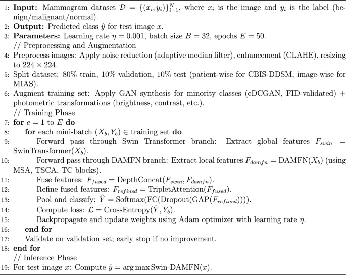
Swin-DAMFN algorithm for breast cancer classification
Computational complexity
The computational complexity of the proposed Swin-DAMFN model is analyzed in Big O notation, considering its dual-branch architecture. The Swin Transformer branch, which processes the input mammogram of size \(H \times W\) divided into \(h \times w\) patches (where \(h = H/4\), \(w = W/4\) initially), achieves a complexity of \(\mathcal {O}(4hwC^2 + 2M^2 hw C)\) per block, where C is the feature dimension and M is the fixed window size (typically 7). Due to the hierarchical shifted-window mechanism, the overall complexity scales linearly with image size, \(\mathcal {O}(HW)\), as detailed in the original Swin Transformer work66.
This is a significant improvement over standard ViT, which exhibits quadratic complexity \(\mathcal {O}((HW/P^2)^2)\) with respect to the number of patches (patch size P), making Swin more efficient for high-resolution medical images. The DAMFN branch, a CNN-based network, comprises multiple convolutional blocks (MSA, TSCA, and TC). Each convolutional layer has a complexity of \(\mathcal {O}(HW K^2 C_{in} C_{out})\) for standard convolutions, where K is the kernel size. Depthwise separable variants (e.g., in MSA) reduce this to \(\mathcal {O}(HW (C_{in} + C_{out}/g + K^2 C_{in}/g))\) with group size g, approximating \(\mathcal {O}(HW C^2)\) across layers. Attention modules like CBAM and Triplet Attention add \(\mathcal {O}(HW C + C^2)\), which is negligible compared to the convolutions. Overall, DAMFN maintains \(\mathcal {O}(HW C^2)\) complexity, similar to conventional CNNs like ResNet, but with enhanced multi-scale efficiency due to parallel pathways.
The full Swin-DAMFN model, operating the branches in parallel before attention-guided fusion (adding \(\mathcal {O}(HW C)\) via Triplet Attention on concatenated features), has an overall complexity of \(\mathcal {O}(HW C^2)\). This is comparable to standalone CNNs but more efficient than pure ViT (\(\mathcal {O}(H^4)\) scaling), balancing global and local feature extraction without excessive computational overhead. Empirical runtime on a single NVIDIA RTX 3090 GPU confirms this efficiency, with inference times of approximately 12 ms per image.


