Skin disease diagnostics through federated transfer learning on heterogeneous data

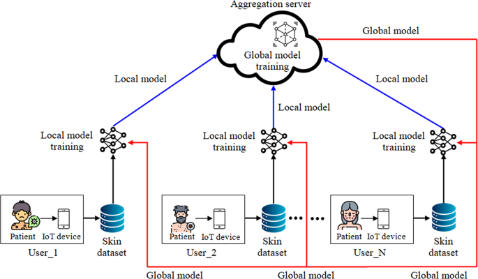
This section presents a resource-efficient FL outline for the recognition and classification of skin illnesses. IoT-enabled devices at different locations collect skin disease images from patients and store them locally. The overall structure of data collection for skin disease diagnosis using FL is shown in Fig. 1. By using distributed data to enhance the accuracy of ML/DL models, it facilitates more effective diagnosis of skin conditions. Figure 2 illustrates the conceptual framework for skin disease diagnosis using four distinct strategies: federated transfer learning, feature extraction with FL, feature extraction with transfer learning, and transfer learning alone. In this framework, images of skin conditions are collected from patients across different locations and stored locally to maintain data confidentiality. Once data collection is complete, pre-processing methods—such as resizing, grayscale conversion, and sharpening—are pragmatic to reduce noise and enhance image quality. Following pre-processing, the dataset is analyzed using four methods.

1. 1.

   The first method, transfer learning, employs DNN to fine-tune a pre-trained model for skin disease classification.

2. 2.

   The second method combines feature extraction and transfer learning, where pre-trained models like DenseNet, VGG19, Xception, and UNet are used to extract features, which are then used for DNN-based classification.

3. 3.

   The third method integrates FL and feature extraction, enabling distributed clients to collaboratively train models on both IID and non-IID datasets while ensuring strong performance and privacy.

4. 4.

   The fourth method —federated transfer learning—uses FL in conjunction with transfer learning to build a global model from dispersed data while preserving patient privacy.

The proposed framework offers a secure, scalable solution to modern healthcare challenges by leveraging ML/DL methodologies in a decentralized setting.

FL with IID and non-IID datasets

Federated learning (FL)³³ model arrange statistics and secrecy while dealing the hitches of exercise representations above a net of detached plans. The parameters or gradients of these locally trained replicas are then collective to generate a global model. By keeping the system exercise course as adjacent to the statistics bases as likely, FL model aims to safeguard data privacy. FL model is therefore, a good optimal for submissions where secrecy is important, mainly when working with complex numbers, geographically detached evidence, or campaigns with partial possessions or erratic network connectivity. FL model has attracted a lot of consideration and research in a range of actual submissions, despite its challenges, particularly in the security domain³⁴. The data-privacy-conscious industries like healthcare and finance employ FL model more frequently to overawe the confines of federal data storage. Without disclosing private patient information to outside servers, FL model enables cooperative model training in the medical field to identify illnesses³⁵. FL model employs IID datasets, which have a uniform and balanced distribution of data among devices³⁶, and Non-IID datasets, which have an uneven and different distribution of data between devices³⁷. Real-world scenarios with inconsistent data from several sources are often reflected in non-IID databases. FL model enables resident strategies to maintain their discrete and assorted documents though attractive a universal system, even in cases when data is not disseminated evenly.

Model training using transfer learning

In deep learning, transfer knowledge is the procedure of applying the information acquired from previously trained models to new and related situations. The key idea is to shift the focus from a large-dataset-trained model to a different-but-related goal that requires fewer labeled instances. The substantial monetary outlay needed to train intricate variables in DL models drives transfer learning. TL has becoming more and more popular in this business for good reason, and it’s easy to incorporate into real-world applications. This process retrains a trained network using just the final classification layer’s parameters by the exercise statistics from the novel mission. This study identifies skin illnesses using transfer learning models, including VGG16, Xception, EfficientNetB3, and MobileNetV2³⁸. By initializing models using learned properties, transfer learning has the advantage of speeding up training and reducing computational and resource costs. CNNs are distinguished by their hierarchical representations and use of convolutional, pooling, dropout, and fully connected layers to extract features from pictures. The transmission learning model has already recognized useful traits and trends across a range of data, serving as a knowledge base. Applying the model to new work only improves the top layers; the lower layers retain all of their learnt information. Initially, transfer learning models only train on low-level structures, keeping all additional layers fixed. While training on a new dataset, transfer learning models often have their remaining layers updated or adjusted. By enabling the model to derive higher-level features pertinent to the new data distribution, altering these layers may enhance the model’s performance.When enhancing a transfer learning model, it’s important to pick your layers wisely and strike a balance between relying on prior knowledge and learning from fresh data.he empirical source distribution \(\hat{Y}\) is specified as \(\hat{Y} = \left\{ {\hat{Y}_{1} ,\hat{Y}_{2} , \ldots ,\hat{Y}_{K} } \right\}\), while the source circulation Y for multi-source transfer learning is definite as \(Y = \{ Y_{1} ,Y_{2} , \ldots ,Y_{K} \}\), where \(I_{k}\) represents the distribution of the K-th basis domain. For the set of hypothesis functions I that map P to Q, let (⋅,⋅) ∶Q × Q → R + represent the loss function. The next is the definition of the q-Discrepancy distance discY between two distributions, \(I_{1}\) and \(I_{2}\):

where \(I_{{x_{i} }} (i,F_{{\Gamma_{i} }} ): = e_{{p\sim x_{i} }} [(i(p),F_{{\Gamma_{i} }} (p))]\). \(F_{{Y_{1} }}\) And \(F_{{Y_{2} }}\) denotes the labeling meaning for the delivery \(Y_{1}\) and \(Y_{2}\), respectively. The empirical optimal problem of f may be clearly shown as follows, given a hypothesis class of real-valued functions f and a set of training data samples \(T = \left( {t_{1} , \ldots ,t_{a} } \right)\):

where \(\varepsilon = (\varepsilon_{1} , \ldots ,\varepsilon_{a} )\), \({\mathcal{E}}_{h}\) are the Rademacher random variables \(X(\varepsilon_{h} = – 1) = X(\varepsilon_{h} = 1) = 0.5\). Let I be a set of theory functions i(⋅) that map the first s-time step efforts \(\{ P_{1} ,P_{2} , \ldots ,P_{5} \} \in r^{{c_{n} \times 5}}\) to the s-time-step output \(q_{s} \in r^{{c_{q} }}\). Using the set I and the distribution X, a new hypothesis function set \(l_{I}\) is distinct as follows:

where the initial t-time-step inputs \(p \in r^{\rho }\) are mapped to [0, 1] by the loss purpose \(l(i(p),F_{X} (p)) \in l_{I}\), an \(l_{R}\)-Lipchitz function associated with the RNN hypothesis. The following equality holds with chance at least 1 − δ over X for every i ∈ I given a dataset of m samples \(\hat{X} = \left( {p_{h} = q_{h} } \right)_{s – 1}^{s}\) h = 1…that is taken from the domain X:

Particular a dataset of K divisions with \(a_{g}\) examples h = 1…\(a_{g}\) strained from several basis areas \(Y_{g}\) for g = 1… K, the next equivalence grips with chance no less than 1 − δcompleted \(Y = \{ Y_{1} ,Y_{2} , \ldots ,Y_{K} \}\) for all i ∈ I:

The next variation grips for \(Y_{g}\) with chance no less than 1 − δ∕K using δ∕K in its place of δ for g = 1, … K.

samples \(\hat{Q} = \left( {p_{h}^{g} \cdot q_{h}^{g} } \right)_{s – 1}^{S}\),h = 1,…, \(a_{g}\), from the basis domain \(Y_{g}\) for g = 1, …, K, and set of data samples \(\hat{X} = \left( {p_{h} = q_{h} } \right)_{s – 1}^{s}\),h = 1,…,a, drawn from the aim area X. The triangle inequality and the definition were used to compute the Q-discrepancy distance. The following equation can further constrain the major component in the next line with a probability of at least 1 − δ over X, according to the goal function.

Additionally, the bound for \(Disc_{Q} (Y,\hat{Y})\)

Let me be a private of the theoretical purpose i(⋅) that translates the concept of the RNN to the output of the s-th step. The following difference grips with a chance of at least 1 − δ: Set a dataset of K subsections with samples \(\hat{Q} = \left( {p_{h}^{g} \cdot q_{h}^{g} } \right)_{s – 1}^{S}\) h = 1,…, to from the base domain \(Y_{g}\) for g = 1,…, K, and a set of data samples \(\hat{X} = \left( {p_{h} = q_{h} } \right)_{s – 1}^{s}\), h = 1,…,a, pulled from the objective area X.

The triangle inequality condition and the discrepancy distance concept may be used to get the following inequality.

Q-discrepancy distance and characteristics of empirical source distribution \(\hat{Y} = \left\{ {\hat{Y}_{1} ,\hat{Y}_{2} , \ldots ,\hat{Y}_{K} } \right\}\) defined as follows.

Lastly, the inequality that follows may be obtained using

The empirical error of the function i as evaluated on the experimental multi-source area \(\hat{Y}\) is represented. \(\hat{X}\) And \(\hat{Y}\) is Q-discrepancy distance is the second term. The function set I on the empirical basis domain \(\hat{Y}\) and the empirical goal domain \(\hat{X}\) has a Rademacher difficulty term that is the third and fourth terms, respectively. The final two elements show the probability terms, which are based on the assurance level δ and the quantity of data samples.

Feature extraction using pre-trained architectures

A key component of DL models that enables effective use of a pre-conditioned neuronal system’s abilities is feature extraction. Among the several layers in these networks that are especially built to extract essential characteristics for tasks like object identification and localization are convolutional and pooling layers. To might change the learning rate, add layers, and variation the sum of neurons in every stratum, and so on to advance our systems. These methods provide significant time and computing resource savings. Pre-trained replicas that have been trained on huge datasets are effective feature extractors. System performance can be improved by selecting the appropriate feature extractor. DenseNet, VGG19, Xception, and UNet were among the pre-trained models³⁹ used which are used to extract the properties of the second-to-last layers. The resulting attributes are then used to classify skin illnesses in FL with IID and Non-IID databases. By allowing remote devices to work together by sharing these derived features for model training, they excel at extracting meaningful patterns from high-dimensional image data, such as lesions’ shape, colour, texture, and edge details, which are critical for diagnosing skin conditions.

Classification using dense neural network (DNN)

Dense neural network (DNN) is highly effective in performing complex classification tasks and learning intricate data representations⁴⁰. A DNN can learn hierarchical features from input data because it has several completely linked layers, with each neuron in one layer connected to every other neuron in the layer above. In this context, DNNs are particularly advantageous. As the input features propagate deeper into the network, higher layers extract more abstract and disease-specific patterns, enabling accurate differentiation between various skin conditions. To simulate intricate relationships in the data, each layer of a DNN applies a weighted sum and then a non-linear activation function.The model is trained using supervised learning with labeled datasets, optimizing weights via backpropagation and gradient descent to minimize classification error. The architecture’s ability to learn deep, abstract features makes it well-suited for skin disease diagnosis, where subtle variations in texture, color, and lesion shape can significantly affect classification accuracy. By leveraging the dense connectivity of DNNs, the system achieves robust performance in automated dermatological analysis. The architecture consists of three main layers: the input, hidden, and the output layer. The input layer is the first point of contact for the model and receives raw data, which, in the context of skin disease classification, typically includes a feature vector derived from skin images. The hidden layers form the core computational engine of the DNN, where each layer applies a weighted sum followed by a non-linear ReLU activation function. The first hidden layer focuses on detecting low-level features like edges, spots, and gradients, which serve as fundamental building blocks in image recognition. Subsequent intermediate layers learn to combine these low-level cues into more complex structures such as textures, shapes, and boundary patterns that are often characteristic of specific skin conditions. The model’s depth and width significantly influence its ability to generalize across diverse cases, although deeper networks may require larger datasets and robust regularization to mitigate overfitting. The output layer gives the classification result, typically using a softmax activation function to generate chances for each class.The input and output feature maps of a precise layer can be characterized as \(P \in r^{I \times Z \times H}\) and \(Q \in r^{I \times Z \times O}\), where I, Z, H, and O represent the height, width, and number of channels, individually. The convolutional filters are embodied as \(D \in r^{I \times O}\). In group involvedness, the feature maps P, Q , and the filters D are separated into G distinct groups. Group convolution is characterized in the calculations below. Here ⊗ characterizes 2D convolution.

The depth-dependent convolution used in the DNN module allows for the extraction of localized features while preserving the spatial scale of the data. The subsequent point-wise dense vector further improves the replica’saptitude to acquiremultifaceted representations by combining features from different channels, allowing for richer information encoding. Depth convolution and point convolution is describes as follows.

Here Z denotes the difficulty kernel, q denotes the contributionarticle map, h and g are the dimensions of the input feature map, K and L are the dimensions of the output feature map, and m denotes the number of channels. Triple attention (TA) improves the replica’scapability to recognize and discriminate different characteristics. Each branch is used to analyze the input tensor (χ ∈ RC × I × Z) in different ways, which improves the model’s complex shapes. In each branch, the input tensor undergoes rotation, followed by W-union and convolution operations, which help extract dimensional correlations between height and channel dimensions. The W-pool function is given by the following relation.

By capturing key interactions between features at dissimilarbalances and locations, TA improves the replica’s ability to identify subtle patterns essential for accurate classification. The final refined feature map is generated by averaging the refined tensors generated by each branch.

whereσ represents the sigmoid function of each objective while \(\psi_{1}\),\(\psi_{2}\) and \(\psi_{3}\) denotes the average two dimensional convolutional layers definite by kernel size K in the three twigs of triplet courtesy.

where \(\omega_{1}\), \(\omega_{2}\), and \(\omega_{3}\) represents the three-dimensional attention weights \(q_{1}\) and \(q_{2}\) which ensures that TA effectively captures spatial and channel dependencies. The working process of skin disease diagnosis using DNN is summarized in Algorithm 1.