Machine Learning “Advent Calendar” Day 3: GNB, LDA, and QDA in Excel

Using k-NN (k-NN regressor and k-NN classifier), we can see that the k-NN approach is very simple. It keeps the entire training dataset in memory, relies on raw distances, and does not learn structure from the data.

We have already started improving the k-NN classifier and in today's article we will implement the following different models:

GNB: Gaussian Naive Bayes
LDA: Linear Discriminant Analysis
QDA: Quadratic Discriminant Analysis

For all these models, the distribution is assumed to be Gaussian. Therefore, at the end we will also present an approach to obtain a more customized distribution.

If you read the previous article, you may have the following questions:

What is the relationship between LDA and QDA?
What is the relationship between GBN and QDA?
What if the data is not Gaussian at all?
How can I get a customized distribution?
What is linear in LDA? What is quadratic in QDA?

You can use this Excel/Google sheet while reading the article.

GNB, LDA, and QDA in Excel – Image by author

Nearest center of gravity: What is this model?

Let's quickly summarize what we already started yesterday.

We introduced a simple idea. Computing the average of each continuous feature within a class collapses the class to a single representative point.

This will give you the nearest centroid model.

Each class is summarized by its centroid, the average of all feature values.

Now let's think about this from a machine learning perspective.
The process is usually divided into two parts. training step and Hyperparameter tuning step.

For the nearest centroid case, you can draw a small “model card” to understand what this model actually is.

How is the model trained? By computing one mean vector for each class. Nothing more.
Are missing values handled? yes. The centroid can be calculated using all available (non-empty) values.
Does scale matter? Yes, definitely because the distance to the centroid depends on the units of each feature.
What are hyperparameters? None.

I mentioned that the k-NN classifier is not a real model, so it may not be a real machine learning model.

In the case of the nearest neighbor centroid, it is not really a machine learning model because it cannot be adjusted. So what about overfitting and underfitting?

Well, the model is so simple that it cannot memorize noise in the same way as k-NN.

Therefore, the nearest centroids only tend to be: underfit This is because if the classes are complex or not well separated, a single centroid cannot capture the complete structure.

Understand the shape of a class with one feature: Adding variance

Now, in this section, we will only use one continuous feature and two classes.

Previously, we used only one statistic (average) per class.
Now let's add the second piece of information. dispersion (or equivalent standard deviation).

This shows how “dispersed” each class is around the mean.

A natural question immediately arises: which distribution should I use?

The most intuitive answer is to calculate 1 difference per classbecause the spreads can be different for each class.

But there is another possibility. You might be able to calculate it. One variance common to both classestypically computed as a weighted average of the class variances.

It feels a little unnatural at first, but you'll later see that this idea leads directly to LDA.

Therefore, the table below shows everything you need for this model, and in fact for both versions of the model (LDA and QDA).

Number of observations in each class (to weight the classes)
Average of each class
Standard deviation for each class
common standard deviation across both classes

These values completely define the entire model.

Once we have the standard deviation, we can construct a more sophisticated distance: the distance to the centroid. Divided by standard deviation.

Why do we do this?

This gives us the distance, so scaled It depends on how mutable the class is.

If the standard deviation of a class is large, it is not surprising that the center of gravity is far away.

If the standard deviation of a class is very small, even small deviations can be important.

This simple normalization turns the Euclidean distance into something a little more meaningful describing the shape of each class.

This distance was introduced by Mahalanobis, so we call it Mahalanobis distance.

You can now perform all these calculations directly in your Excel file.

The formula is simple and with conditional formatting you can clearly see how the distance to each center changes and how the scaling affects the result.

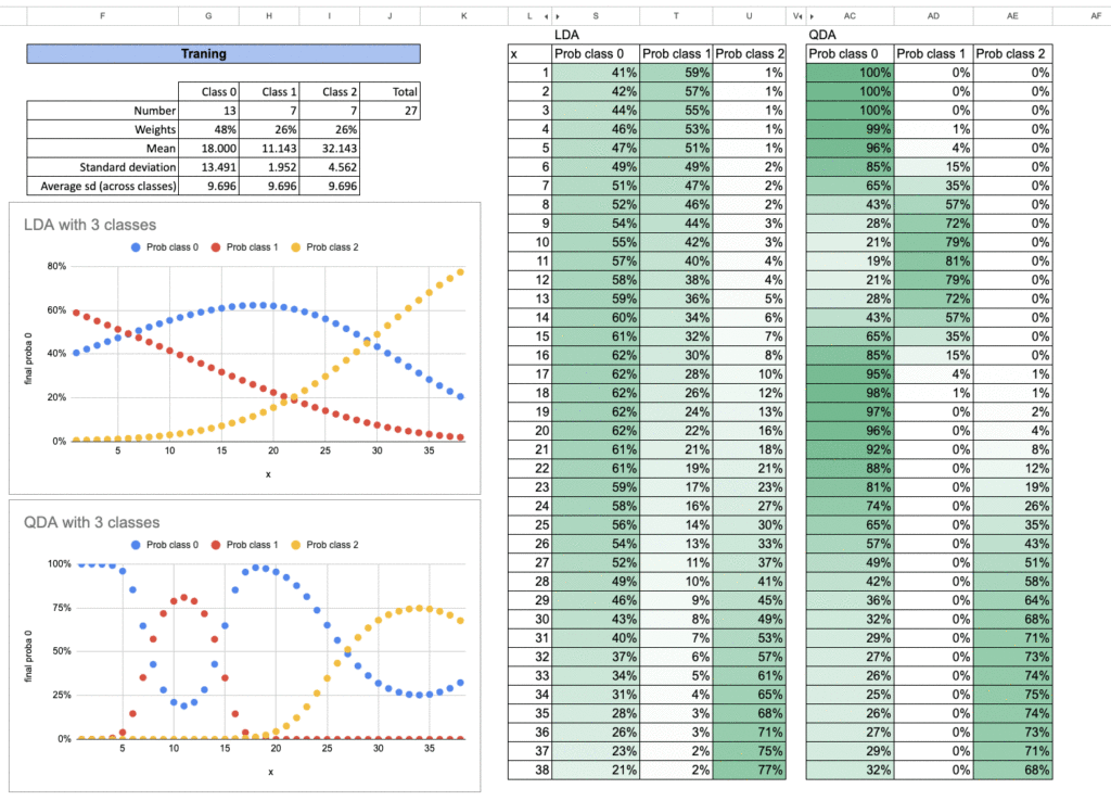
Now let's create some plots, always using Excel.

The figure below shows the complete progression of how to start from the Mahalanobis distance, proceed to the likelihood under each class distribution, and finally obtain the probability predictions.

LDA vs. QDA, what do you see?

With just one feature, the difference is very visible.

for LDAthe separation on the x-axis is always divided into two parts. This is why this method is called linear Discriminant analysis.

for QDAeven if there is only one feature, the model will generate: two Cut a point on the X axis. In higher dimensions, this becomes the boundary of the curve, quadratic function. Therefore, the name is quadratic function Discriminant analysis.

You can also directly change the parameters and see how they affect the decision boundary.

Changes in the mean and variance change the frontier, and Excel makes it very easy to visualize these effects.

By the way, doesn't the shape of the LDA probability curve remind you of a model you know for sure? Yes, it looks exactly the same.

You already know which one is which, right?

But the real question here is, are they? Really Is it the same model? If not, how are they different?

You can also study cases in three classes. You can try this out yourself as an Excel exercise.

Here are the results: Repeat the exact same steps for each class. The final probability prediction then simply adds up all possibilities and calculates the probability of each.

Again, this approach is also used in another well-known model.
Do you know which one? This is much more familiar to most people, which shows how closely related these models really are.

If you understand one of them, you will automatically understand the others better.

2D class shape: variance only or covariance too?

I won't discuss one feature because it has no dependencies. Therefore, in this case, QDA behaves exactly like Gaussian Naive Bayes. Because we usually allow each class to have its own variance, which is completely natural.

Differences emerge when you move to more than one feature. At that point, we differentiate the cases of how the model handles it. covariance between functions.

Gaussian Naive Bayes makes one very strong simplifying assumption.
Functions are independent. this is the reason for the word naive By that name.

However, LDA and QDA do not make this assumption. They allow interactions between features and this is what generates linear or quadratic boundaries in high dimensions.

Let's practice with Excel!

Gaussian naive Bayes: no covariance

Let's start with the simplest case, Gaussian Naive Bayes.

Therefore, there is no need to calculate covariance at all since the model assumes that the features are independent.

To illustrate this, let's look at a small example containing three classes.

QDA: each class has its own covariance

For QDA, we need to calculate the covariance matrix for each class.

And once we have that, we also need to calculate its inverse, as it is used directly in the distance and likelihood formulas.

Therefore, there are a few more parameters to calculate compared to Gaussian Naive Bayes.

LDA: all classes share the same covariance

For LDA, all classes share the same covariance matrix, which reduces the number of parameters and makes the decision boundary linear.

Although the model is simpler, it is very effective in many situations, especially when the amount of data is limited.

Customized Class Distributions: Beyond Gaussian Assumptions

So far we have only discussed Gaussian distributions. That's because of its simplicity. You can also use other distributions. So it's very easy to make changes, even in Excel.

In reality, data usually does not follow a perfect Gaussian curve.

Almost every time I explore a dataset, I use an empirical density plot. Instantly visualize how your data is distributed.

and, Kernel Density Estimator (KDE) It is often used as a non-parametric method.

However, in practice, KDE is rarely used as a complete classification model. This is not very convenient, and its prediction often depends on bandwidth selection.

And what's interesting is that this kernel idea comes up again when discussing other models.

Therefore, although it is shown here primarily for exploration, it is an essential building block in machine learning.

KDE (Kernel Density Estimation) in Excel – Image by author

conclusion

Today we started with a simple average and gradually followed the natural path to a full probabilistic model.

Nearest centroid compresses each class to one point.
Gaussian Naive Bayes adds the concept of variance and assumes feature independence.
QDA gives each class its own variance or covariance
LDA simplifies the shape by sharing covariances.

It turns out you can also go outside of the Gaussian world and explore customized distributions.

All these models are connected by the same idea. New observations belong to the most similar class.

The difference is how we define similarity by distance, variance, covariance, or complete probability distribution.

For all of these models, you can easily perform the following two steps in Excel:

The first step is to estimate the parameters. This can be considered as training the model.
An inference step that calculates distances and probabilities for each class.