In this five-day machine learning “advent calendar,” we considered five models (or algorithms), all based on distance (local Euclidean distance, or global Mahalanobis distance).
It’s time to change your approach, right? We will discuss the concept of distance later.
Today we're going to talk about something completely different: decision trees.

Introduction with a simple dataset
Let's use a simple dataset with just one continuous feature.
As always, the idea is that you can visualize the results yourself. Now you have to figure out how to get your computer to do it.

For the first split, you can visually infer that there are two possible values, one around 5.5 and one around 12.
Now, the question is which one to choose.
This is exactly what we are going to explore. How do we determine the value of the first split in our implementation in Excel?
Once you have determined the value for the first split, you can apply the same process to subsequent splits.
Therefore, Excel only implements the first split.
Decision tree regressor algorithm principles
I wrote an article called Always Differentiate the Three Steps of Machine Learning to Learn Machine Learning Effectively and Let's Apply Those Principles to Decision Tree Regressors.
So for the first time we have a “true” machine learning model with non-trivial steps in all three.
What is the model?
A model here is a set of rules for partitioning a dataset and assigning a value to each partition. which one? Average value y of all observations in the same group.
Therefore, a k-NN uses the mean of the nearest neighbors (observations that are similar in terms of a feature variable) to predict, whereas a decision tree regressor uses the mean of a group of observations (similar in terms of a feature variable) to make predictions.
The process of fitting or training a model
For decision trees, this process is also called growing the tree to full size. For decision tree regressors, the leaves contain only one observation, so the MSE is 0.
Growing a tree consists of recursively dividing the input data into smaller chunks or regions. You can calculate predictions for each region.
For regression, the prediction is the average of the target variable over the domain.
At each step in the construction process, the algorithm selects features and split values that maximize one criterion. For regressors, the mean squared error (MSE) between the actual value and the prediction is often used.
Tuning or pruning the model
For decision trees, the general term for model tuning is also known as pruning, which can be thought of as removing nodes and leaves from a fully grown tree.
It is also equivalent to saying that the construction process stops when criteria such as the maximum depth of each leaf node or the minimum number of samples are met. These are hyperparameters that can be optimized during the tuning process.
reasoning process
Once a decision tree regressor is constructed, it can be used to predict the target variable for new input instances by applying rules and traversing the tree from the root node to the leaf nodes corresponding to the input feature values.
The predicted target value of an input instance is the average of the target values of training samples that fall into the same leaf node.
Implementing the first split in Excel
Follow the steps below:
- List all possible splits
- Compute the MSE (Mean Squared Error) for each fold.
- Select the split that minimizes the MSE as the best next split.
all possible divisions
First, we need to list all possible splits that are the average of two consecutive values. There is no need to test more values.

MSE calculation for each possible split
As a starting point, you can calculate the MSE before partitioning. This also means that the prediction is just the average value of y. And MSE is equal to the standard deviation of y.
The idea here is to find a split such that the MSE with the split is lower than before. It is possible that splitting does not significantly improve performance (or reduce MSE), in which case the final tree will be trivial, i.e., the mean value of y.
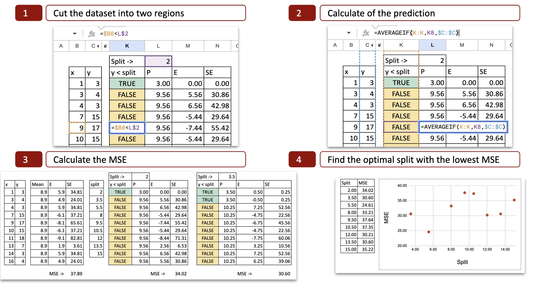
For each possible split, we can calculate the MSE (Mean Squared Error). The figure below shows the calculation for the first possible split (x = 2).

You can check the calculation details.
- Split the dataset into two regions. For the value x=2, there are two possibilities x<2 または x>2 is determined, so the x-axis is divided into two parts.
- Calculate predictions. Compute the mean of y for each part. That is the potential prediction of y.
- Calculate the error. Next, compare the prediction to the actual value of y.
- Calculate the squared error: You can calculate the squared error for each observation.

optimal split
For each possible split, do the same to obtain the MSE. Excel allows you to copy and paste formulas. The only values that change are the divisible values of x.

Next, if we plot the MSE on the Y-axis and the possible splits on the X-axis, we can see that there is a minimum value of MSE at x=5.5. This is exactly the result I got with my Python code.

Exercises I want to try
Now you can play with Google Sheets.
- As you change the dataset, MSE updates to show you the best cuts.
- You can introduce category features
- You can try looking for the next split
- You can change the criteria instead of MSE. You can use absolute error, Poisson, or friedman_mse as shown in the DecisionTreeRegressor documentation.
- You can change the target variable to a binary variable. Typically this would be a classification task, but since 0 or 1 are also numbers, the MSE criterion can still be applied. But if we want to create a good classifier, we need to apply the usual criteria Entroy or Gini. That's for the next article.
conclusion
Using Excel, you can implement a single split to gain more insight into how decision tree regressors work. Even if you didn't create a complete tree, it's still interesting because the most important part is finding the best split among all possible splits.
One more thing
Did you notice anything interesting about how features are handled between distance-based models and decision trees?
For distance-based models, everything must be numeric. Continuous features remain continuous, and categorical features must be converted to numbers. The model compares points in space, so everything must lie on the numerical axis.
Decision trees do the opposite. cut Divide features into groups. Continuous features become intervals. Category features remain categories.
Are there missing values? It's just another category. There is no need to assign it first. Trees, like other groups, can naturally handle this by sending all “missing” values down one branch.


