Test-setup
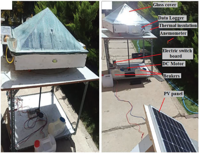
Modified pyramidal solar still with rotational mechanism to enhance the condensation and evaporation processes was designed and constructed. The system utilizes a pyramidal configuration operating at a rotational speed of 1 rpm. The experimental setup is equipped with rotating wheels connected to a central shaft, which is driven by a 6 W DC motor. Figure 1and 2 illustrate the experimental configuration. The tests were performed at the University of Science and Technology in Tehran, located at a latitude of 35.44° N and longitude of 51.41° E. Productivity of freshwater was determined hourly and collected utilizing a measuring jar for distilled water to recording total Solar distillation system yield per day2.

Constructed testing apparatus of the pyramidal solar still2.

Illustration of the experimental configuration2.
The factors influencing the performance of the distiller system were recorded and evaluated in the specified time period. The parameters include wind velocity, sun irradiance, ambient temperature, and rotational speed. The configuration of the pyramidal distillation system requires the consideration of parameters including the exposed surface area to solar irradiation. The design specifications feature an absorptive plate of 70 × 70 cm. The basin of water is constructed using 1.5 mm thick galvanized iron, and the cover of pyramid comprises four clear glass panels, each 4 mm in thickness. Feedwater system of the solar still technique consists of a small funnel connected to a floating water buoy in the tank. The data logger, feeding system, and distillated water jug for collection are attached to the exterior perimeter of the solar still. The examination setup connected to a rotating shaft driven. A solar panel was utilized to eliminate the need for fossil-based energy systems. The pyramid-shaped solar still follows the proportions of prior models, featuring a tilt angle of the glass cover that corresponds using the local latitude2.
Measuring tools
Solar distiller performance is often evaluated on numerous critical features, involving solar irradiance, temperature, distillated volume, and air speed. The configuration is supplied with several measurement instruments essential for collecting data and analysis. This equipment is included into the monitoring system and document the important variables through the experiential tests. Appropriate instruments are employed to determine those features via experimentation30. A solar meter is utilized to measure irradiation values at different daily interval. Determinations of temperatures were obtained using thermocouple wires. Furthermore, the anemometer is employed to measure air velocity. The solar distiller yield is assessed utilizing the accurate balance mechanism. Table 2 represents comprehensive details of the instruments employed in the experimental analysis2.
System efficiency
The performance of several solar distiller models has been evaluated using energy and exergy efficiency45. The efficiency depends on the water output of the solar distiller and the heat transfer mechanism within it. The condensation rate indicates the distillate yield of freshwater generated by the solar still system, additionally referred to as the hourly or daily the system productivity. The overall thermal efficiency of a solar still unit in passive and active operation types, as presented by Kabeel et al.46, allows for the hourly distilled yield of the solar still to be defined as follows in Eq. (1):
$${\dot{\text{m}}}_{{\text{W}}} = \frac{{{\upeta }_{{{\text{th}}}} \times A \times \sum {{\text{I}}\left( {\text{t}} \right) \times 3600} }}{{{\text{h}}_{{{\text{fg}}}} }}$$
(1)
where \(\eta_{th}\) is presented as the thermal efficiency, \({\text{h}}_{{{\text{fg}}}}\) is the latent heat of vaporization, \({\text{I}}\left( {\text{t}} \right)\) and \(A\) are the average daily solar radiation, the total area respectively. According to Eq. (2), the thermal efficiency over the day is then47:
$${\upeta }_{{{\text{th}}}} = 0.727 – 2.88 \times 10^{2} \frac{{\text{T}}}{{{\text{I}}\left( {\text{t}} \right)}}$$
(2)
where \({\text{I}}\left( {\text{t}} \right)\) is the mean daily solar irradiance on the still from sunrise to sunset. T is the time period.
Besides, \(h_{fg}\) is determined by the water temperature (\(T_{W}\)), by Emad et al.48 as follows in Eq. (3):
$${\text{h}}_{{{\text{fg}}}} = 10^{3} \times \left[ {2501.09 – 2.40706 \times {\text{T}}_{{\text{W}}} + 1.192217 \times 10^{ – 3} \times {\text{T}}_{{\text{W}}}^{2} – 1.5863 \times 10^{ – 5} \times {\text{T}}_{{\text{W}}}^{3} } \right]$$
(3)
\({\text{T}}_{{\text{W}}}\) is proportional to the ambient temperature in each season.
Deep neural networks
LSTM model
LSTM, a specialized type of recurrent neural network (RNN), is developed to address the vanishing gradient issue. Its sophisticated architecture allows LSTM networks Aimed at accurately capturing and processing long-term dependencies in sequential data. These networks are extensively utilized across different sectors, involving speech recognition, challenges including sequence modeling and natural language processing. The primary advancement of LSTM is the incorporation of memory cells and gating processes. In the LSTM architecture illustrated in Fig. 3, the forgetting gate eliminates input data while maintaining critical data49. It generates a vector ranging from 0 to 1 to ascertain which data in the cell state Ct−1 should be preserved. Input control gate modifies xt using the sigmoid function and ht−1 using the tanh function to collectively update the cell state. Output control gate comprises two components: The output at time t, ot, along with the updated hidden state ht, with ot determined by xt and oht-1. The detailed operational concept is articulated by Eqs. (4) to (9) 50:
$${\text{f}}_{{\text{t}}} = {\upsigma }\left( {{\text{W}}_{{\text{f}}} .\left[ {{\text{h}}_{{{\text{t}} – 1}} ,{\text{x}}_{{\text{t}}} } \right] + {\text{b}}_{{\text{f}}} } \right)$$
(4)
$${\text{i}}_{{\text{t}}} = {\upsigma }\left( {{\text{W}}_{{\text{i}}} .\left[ {{\text{h}}_{{{\text{t}} – 1}} ,{\text{x}}_{{\text{t}}} } \right] + {\text{b}}_{{\text{i}}} } \right)$$
(5)
$${\text{g}}_{{\text{t}}} = {\text{tanh}}({\text{W}}_{{\text{g}}} .\left[ {{\text{h}}_{{{\text{t}} – 1}} ,{\text{x}}_{{\text{t}}} } \right] + {\text{b}}_{{\text{g}}}$$
(6)
$${\text{C}}_{{\text{t}}} = {\text{g}}_{{\text{t}}} \times {\text{i}}_{{\text{t}}} + {\text{C}}_{{{\text{t}} – 1}} \times {\text{f}}_{{\text{t}}}$$
(7)
$${\text{o}}_{{\text{t}}} = {\upsigma }\left( {{\text{W}}_{{\text{o}}} .\left[ {{\text{h}}_{{{\text{t}} – 1}} ,{\text{x}}_{{\text{t}}} } \right] + {\text{b}}_{{\text{o}}} } \right)$$
(8)
$${\text{h}}_{{\text{t}}} = {\text{o}}_{{\text{t}}} \times \tanh \left( {{\text{C}}_{{\text{t}}} } \right)$$
(9)

The LSTM model structure.
Wf, Wi, Wg and Wo represent the matrix weights of the respective gates, while bf, bi, bg and bo denote the bias terms. The sigmoid activation function, represented by × , and the tanh function are both employed as activation functions in the model.
CNN model
CNNs are classified as a type of feedforward network models that utilize convolutional operations and consist of convolutional layers, pooling layers, and fully connected layers, as seen in Fig. 4. The convolutional layers execute localized operations on small segments of the input information using a convolutional kernel, as indicated in Eq. (10), therefore capturing spatial patterns and characteristics51.
$${\text{F}} \otimes {\text{w}} = \mathop \sum \limits_{{{\text{i}} = 1}}^{{{\text{H}}_{{\text{k}}} }} \mathop \sum \limits_{{{\text{j}} = 1}}^{{{\text{W}}_{{\text{k}}} }} \left( {{\text{F}}\left( {{\text{i}},{\text{j}}} \right).{\text{w}}\left( {{\text{i}},{\text{j}}} \right)} \right)$$
(10)

In the above context, ⨂ signifies convolutional computation, F represents a segment of the input information, while w, Hk, and Wk stand for the convolution kernel weight parameter, height, and width, respectively52.
CNN-LSTM model
A common design for analyzing time-series data is CNN-LSTM, which combines CNN and LSTM networks. This study uses a hybrid approach to feature extraction using the CNN layer and subsequently transmitting them to the LSTM layer. As seen in Fig. 5, the time-sequenced data are first fed toward the feature-extracting convolutional layer in the CNN of features, followed by the pooling layer, which extracts hidden data, and the flatten layer, which decreases the feature dimension. For more time-series modeling and prediction, the gathered feature sequences are then fed into the LSTM. The aggregated features are subsequently fed into the fully connected layer for forecasting. CNN extracts spatial features in time series data, whilst LSTM captures temporal dependencies; this combination leverages the potential of both models, enhancing the modelling and predictive capabilities of time series data53.

The CNN-LSTM model structure.
GRU model
The GRU neural network is a simplified variant of the LSTM, designed to reduce the number of gates while maintaining long-term memory capabilities, effectively addressing the vanishing gradient issue. GRU comprise two gates: the update gate and the reset gate. The former refers the information discarded related to a new input and the update data incorporated, while the next articulates the extent of long-term or prior data discarded by the forget gate. Equations (11) and (13) refer to the reset and forget gates23.
$${\text{z}}_{{\text{t}}} = {\upsigma }\left( {{\upomega }_{{{\text{zh}}}} .{\text{h}}_{{{\text{t}} – 1}} + {\upomega }_{{{\text{zx}}}} .{\text{x}}_{{\text{t}}} + {\text{b}}_{{\text{z}}} } \right)$$
(11)
$${\text{r}}_{{\text{t}}} = {\upsigma }\left( {{\upomega }_{{{\text{rh}}}} .{\text{h}}_{{{\text{t}} – 1}} + {\upomega }_{{{\text{rx}}}} .{\text{x}}_{{\text{t}}} + {\text{b}}_{{\text{r}}} } \right)$$
(12)
$${\text{h}}_{{\text{t}}}{\prime} = \tanh ({\upomega }_{{{\text{xh}}}} .{\text{x}}_{{\text{t}}} + {\text{r}}_{{\text{t}}} {\upomega }_{{{\text{hh}}}} .{\text{h}}_{{{\text{t}} – 1}} )$$
(13)
In Eq. (13), the input data xt and the prior time step data ht-1 are linearly combined, with the various matrices ω being multiplied correspondingly on the right side. Subsequently, the reset gate rt and ωhh. ht−1 are multiplied. Finally, the updated information regarding the present condition is computed using an activation function, often the tanh function54.
$${\text{h}}_{{\text{t}}} = {\text{z}}_{{\text{t}}} .{\text{h}}_{{{\text{t}} – 1}} + \left( {1 – {\text{z}}_{{\text{t}}} } \right){\text{h}}_{{\text{t}}}{\prime}$$
(14)
As per equation (14), the multiplication of zt and ht−1 indicates the conclusive data information retained from the preceding time step. The output and the information retained from the present memory to the long-term memory. correspond to the output ht generated by the final gate unit. Figure 6 illustrates the structure of the GRU.

Evaluation metrics analysis
Various error measuring techniques can assess the precision of models for forecasting. The study suggests utilizing five assessment measures to assess the model accuracy: mean absolute error (MAE), root mean square error (RMSE), square error (MSE), coefficient of determination (R2), mean and coefficient of variance (COV). Equations (15) to (19) are used to determine the five parameters29,43,55,56:
$${\text{MAE}} = \frac{1}{{\text{N}}}\mathop \sum \limits_{{{\text{i}} = 1}}^{{\text{N}}} \left| {{\text{x}}_{{\text{i}}} – {\text{y}}_{{\text{i}}} } \right|$$
(15)
$${\text{MSE}} = \frac{1}{{\text{N}}}\mathop \sum \limits_{{{\text{i}} = 1}}^{{\text{N}}} \left( {{\text{x}}_{{\text{i}}} – {\text{y}}_{{\text{i}}} } \right)^{2}$$
(16)
$${\text{R}}^{2} = 1 – \frac{{\mathop \sum \nolimits_{{{\text{i}} = 1}}^{{\text{N}}} ({\text{x}}_{{\text{i}}} – {\text{y}}_{{\text{i}}} )^{2} }}{{\mathop \sum \nolimits_{{{\text{i}} = 1}}^{{\text{N}}} \left( {{\text{y}}_{{\text{i}}} } \right)^{2} }}$$
(17)
$${\text{RMSE}} = \sqrt {\frac{1}{{\text{N}}}\mathop \sum \limits_{{{\text{i}} = 1}}^{{\text{N}}} \left( {{\text{x}}_{{\text{i}}} – {\text{y}}_{{\text{i}}} } \right)^{2} }$$
(18)
$${\text{COV}} = \frac{{{\text{RMSE}}}}{{{\overline{\text{y}}}}} \times 100$$
(19)


