
This section provides a detailed description of the DXAIB scheme, including the utilized data-set, its pre-processing, the forecasting of breast cancer, and the explainability of the prediction made by the proposed scheme.
Data-set Description
This study used a dataset entitled “Breast Cancer Wisconsin (Diagnostic)” obtained from the UCI ML repository27. The dataset contains a comprehensive collection of 30 clearly defined features, including the mean, standard error, and worst values of 10 specific features (texture, radius, concavity, area, smoothness, compactness, symmetry, perimeter, concave points, and fractal dimension). These features are obtained from ultrasound pictures of a breast mass obtained by fine needle aspiration (FNA). These features delineate the cellular nuclei seen in the photographs. The collection has a total of 569 unique individual samples. The comprehensive dataset provided a solid basis to follow-up analysis since each item comprised several relevant features. The class label functioned as a categorical variable, indicating separate and identifiable groupings. The class label consisted of two well-defined categories, each representing distinct diagnostic results. The category denoted as ‘M’refers to all presently surviving females who have received a diagnosis of breast cancer. Individuals categorized as ‘B’ indicate the lack of breast cancer. The Breast Cancer Wisconsin (BCW) dataset was chosen for several key reasons such as, historical significance and validation of it, its simplicity and interpretability, and it is a clean and well-structured data that make it particularly useful for the development of classification models for breast cancer detection. The BCW dataset has been extensively used and validated in breast cancer research. The dataset contains a comprehensive set of features derived from fine needle aspiration (FNA) of breast masses, focusing on cell characteristics such as radius, texture, and perimeter, which are clinically relevant for identifying malignancies. The dataset’s features are interpretable, making it ideal for initial testing and development of ML models. The BCW dataset is highly structured, with no significant data inconsistencies, which allows for straightforward analysis and model development.
Data Pre-processing
Data preprocessing encompasses many procedures, including cleaning, transformation, and preparation. The aforementioned steps are carried out to ensure the appropriate processing and structuring of the raw data for further analysis. Through the assurance of data consistency and logical progression, this essential process enables rigorous model training and precise predictions. Approaches such as normalization, feature engineering, and managing missing values are employed to improve the usability and efficiency of datasets for training ML models. A scaling methodology was applied to the dataset following rigorous data collection and a thorough feature selection approach. This measure was implemented to maintain consistency and facilitate relevant comparisons of the characteristics. Scaling, or standardization, was used to consistently measure all traits and minimize biases caused by differences in measuring units. The scaling method included subtracting the mean value from each feature and then dividing the resulting value by the standard deviation of the feature. The methodology employed in this work successfully maintained the relative relationships among the various characteristics and conserved the overall organization of the dataset. Statistical scaling techniques provide an equitable and impartial evaluation of the correlations and patterns seen in the dataset. By standardizing all characteristics to a consistent scale, the potential impact of variations in measurement units was reduced, enhancing the study’s trustworthiness. Quantitative representations of categorical data in ‘D’ are obtained via label encoding. Specifically, the target column in ‘D’ comprises categorical values ‘M’ and ‘B’ corresponding to malignant and benign outcomes. The application of label encoding results in assigning the value ‘1’ to the category ‘M’ and the value ‘0’ to the category ‘B’ (algorithm 1: line 3). Label encoding converts categorical data into a format appropriate for various ML approaches. An additional pre-processing stage involves removing superfluous features from the dataset ‘D’ (algorithm 1: lines 4). Following label encoding and feature selection, all occurrences of duplicate data are eliminated from the dataset ‘D’. In present type of critical applications the sensitivity or recall plays a very critical role where no positive case should be predicted as negative case which can eventually lead to fatality later. The used dataset in the present work is having 62.85% of benign cases whereas, 37.15% of malignant cases. So, dataset was biased towards benign class. Thus, Synthetic Minority Over-sampling Technique (SMOTE) which is a data augmentation technique for tabular data-set is used. It created synthetic samples for minority malignant class by interpolating between existing data points. It can enhance recall by generating synthetic examples for the minority class in an imbalanced dataset. Instead of simply duplicating existing instances, SMOTE creates new, synthetic data points by interpolating between nearest neighbors of the minority class. This process expands the feature space of the minority class, helping models learn more diverse patterns and reducing the chance of misclassifying minority instances as negatives.
DXAIB: The Proposed Scheme.
Breast Cancer Detection
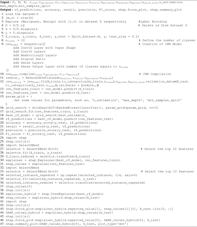
A hybrid ML model that combines Convolutional Neural Networks (CNNs) for feature extraction from tabular dataset with Random Forest for predictive output is developed in this present work. To enhance transparency and interpretability, SHAP (SHapley Additive exPlanations) explainable AI module is included which offers comprehensive insights into the determinants influencing the model’s prediction results. The proposed scheme starts with the loading of data, which is then followed by pre-processing steps. The dataset, denoted as ‘D’, has ‘m’ rows and ‘n’ columns, with ‘m’ indicating the number of rows or data instances and ‘n’ indicating the number of columns or features. Following the successful importation of ‘D’, pre-processing steps are executed as explained in the preceding sub-heading. Subsequently, the data set ‘D’ is partitioned into two subsets: one containing the target feature, including the target class label, and the other including the other features. The proposed DXAIB scheme partitions the dataset into two subsets for training and testing purposes. This is accomplished by using an 80-20 split (algorithm 1, line 7). After the split, data is normalized using the MinMaxScaler function. Following data transformation, the dataset ‘D’ is partitioned into four subsets: X_train, y_train, X_test, and y_test (algorithm 1, line 7). The X_train and y_train datasets are fed into the proposed CNN model, which is a part of the DXAIB scheme. Various layers in the CNN architecture, including convolutional, flattened, dense, and max-pooling layers, include dropout rates. The architectural design of the proposed CNN can be seen in Table 3. Importantly, the proposed CNN is only used for feature learning rather than data categorization. A total of 10 output classes are included in the proposed CNN model. Next, the classification layer of the CNN model is substituted by the RF classifier. The CNN under consideration consists of a total of 10 layers, which include four convolutional layers, one flattened layer, three dense layers, and two max-pooling layers. However, an excessively high number of layers may harm performance, so balancing enhancing accuracy and allocating resources is essential. To address the issue of over-fitting, a dropout rate of ‘0.20’ is applied following every max-pooling and dense layer. After passing through the convolutional and max-pooling layers, the input transforms a planar structure before being sent to the first thick or dense layer. Three thick layers are present, with the first two levels consisting of `512’ and `256’ number of filters, respectively. After the proposed CNN architecture is built, the model is trained using appropriate training data. The validation technique, as shown in algorithm 1, is conducted using validation data with a batch size of ‘64’ epochs and ‘100’ epochs. Before transmitting the data to the RF classification layer, a dense layer is used to modify and restructure it after the training phase. An essential function of this layer is to synchronize the results of the CNN model with the necessary vector shape for the RF layer (algorithm 1: lines 9). Several factors justify the selection of the RF model as the classifier layer, namely its superior accuracy when applied to the dataset compared to other ML techniques. Subsequently, the classification layer generates projections for the resultant class, and the precision of these projections, which measure the model’s adaptive performance, is evaluated. Indeed, the suggested approach is an essential antecedent and decisive factor in directing future evaluations of breast tumor recipients. These patients receive a range of crucial clinical procedures specifically intended to accomplish a thorough assessment. Importantly, our first goal is to determine whether a patient has cancer. Having formulated predictions, this work focuses on clarifying the importance of specific features in identifying patients with various types of cancer.
Explainability
After the class prediction process is completed, the findings or projections are transmitted to the eXplainable Artificial Intelligence (XAI) algorithm for the proposed scheme. Subsequently, the XAI framework is used to provide explanations. The SHAP (SHapley Additive exPlanations) XAI technique is used in this work over others because of its theoretical foundation based on Shapley values, its consistency and additivity, its global and local interpretability, model-agnostic and model-specific variants, its visualization and interpretability, its reliability on feature importance, its ability to capture feature interactions, and its wide adoption and continuous improvement28. It is used in the proposed scheme to engage with the RF layer and provide various explanations. The SHAP approach offers local and global reasons, as shown by the statistical data in the findings section. While the patient may find these explanations unclear, they are crucial for medical practitioners. Upon analysis by a healthcare professional, these clarifications allow them to offer the patient many justifications for a specific disease diagnosis and suggest several alternative diagnostic possibilities (algorithm 1: lines 24-47). After the identification or forecasting stage of the proposed method is finished, the SHAP approach is used to analyze and present many explanations for the predictions produced by the model. SHAP, a well acknowledged and effective method in Comprehensible Artificial Intelligence , is especially developed to uncover the precise influence of certain characteristics on the results produced by a model. The objective of installing SHAP was to achieve accurate and easily understandable explanations in order to improve the transparency of the decision-making framework in the existing system. Prior to implementing SHAP, the proposed ML model predicted outcomes for all patients in the dataset. After that, we calculated SHAP values for all of the model features to see how much of an effect each piece of information had on our prediction technique. The SHAP values measure the effect of each feature’s presence or absence on the model’s output, allowing us to evaluate their relevance. Furthermore, the SHAP scores were meticulously categorized into interpretations for the identified results. More specifically, throughout the stage of some patients, interpretations are generated, offering a comprehensive examination of the main characteristics of each prognosis. Through offering comprehensive explanations customized for each patient, physicians may ascertain the fundamental factors that impacted the diagnosis of each individual patient. By taking this route, they were able to better comprehend how the model arrived at its conclusions. In order to uncover the most prominent trends and patterns, the SHAP values were averaged throughout the sample. Through this aggregate, explanations were extracted on a global scale, revealing underlying features that are regularly linked to forecasts of breast cancer type, whether it is malignant or benign. These global explanations aimed to emphasize overarching patterns in the data and enhance understanding of the system’s functioning in a broader scope. Incorporating SHAP reasoning after the proposed system’s classification phase has shown to be a great help in giving a comprehensive and comprehensible assessment of the scheme’s predictions. The SHAP technique provided clinicians and researchers with profound insights at the individual patient level and on a broader scale. This enabled them to enhance their trust in the model’s evaluations and develop a more profound comprehension of the complex connections between traits and pathological outcomes. Transparency and comprehensibility are crucial for establishing confidence and, hence, determining the practical feasibility and capability of the system to improve breast cancer detection and patient care.


