Polymer design for solvent separations by integrating simulations, experiments and known physics via machine learning

Generation and validation of a computational dataset for solvent diffusivity

We established a high-throughput simulation protocol for calculating solvent diffusivity through polymers, employing classical molecular dynamics (MD) with the open-source LAMMPS package, as detailed in Fig. 1. First, polymer and solvent structures were generated using the open-source Polymer Structure Predictor (PSP)⁵⁹. The polymer chains consist of approximately 150 atoms per chain, with the entire system totaling 4000–5000 atoms, a majority of them operating within a dilute solvent concentration regime, as can be seen in the Supplementary Fig. 1. GAFF2 was employed as the chosen force field. Next, a 21-step equilibration process was employed to ensure that polymers were equilibrated⁶⁰. Afterward, all systems were subjected to an additional 10 ns equilibration in the NPT ensemble, followed by a 200 ns production run in the NVT ensemble²⁹. The Nosé-Hoover thermostat and barostat, with a damping parameter of 100-time steps each, were employed, and a time step of 1 fs was used in all MD simulations. Post-simulation, the diffusivity of the solvent in the Fickian regime was estimated based on mean square displacement analysis for all atoms and averaged for that molecule. Thus the solvent diffusivity (D) is then calculated as:

where N is the number of solvent molecules, t is the simulation time, r_i(t) is the position vector of the solvent at time t, and r_i(0) is the position vector at the initial time 0.

Since the diffusion coefficient D is ideally determined in the limit as t approaches infinity, simulations were run for sufficiently long periods to ensure that the diffusion properties do not vary significantly over time. We ensured that diffusivities are estimated in the Fickian regime by verifying that the slope of the log displacement-log time plot remains close to one. If the slope value is outside the range of 0.95-1.05, the diffusivity runs are excluded from subsequent calculations. Additionally, the standard block average method was used to estimate the simulated uncertainty from 10 blocks⁶¹. The diffusivity simulations were conducted as a function of solvent concentration and temperature. Using the simulation pipeline outlined above, diffusivity calculations were first conducted for polymer-solvent pairs with available experimental diffusivity data, as shown in Fig. 1. For 376 experimental systems across 18 polymers and 45 solvents, a coefficient of determination (R²) of 0.63 was observed, indicating an acceptable correlation between experimental and simulated data^{62,63,64,65,66,67,68,69,70,71,72,73,74,75}. Although the simulated results do not fully align with the experimental data due to inherent limitations in the force field and simulation protocol, the observed qualitative correlation is expected and sufficient for our objective of downstream multi-task machine learning models. After validating the correlation between experimental and simulated values for the 376 systems, the computational diffusivity dataset was expanded beyond the limited experimental space, resulting in a total of 623 systems, comprising 91 polymers and 69 solvents. This expansion of the simulated space is aimed to enhance the generalizability of the downstream multi-task ML model by broadening chemical space coverage, enabling it to learn from a more diverse dataset and make more accurate predictions beyond the constraints of the limited experimental data^29,39,40. Additional details on the simulation protocol can be found in the Supplementary Information (sections 2 and 3).

Data augmentation

Building larger and more diverse datasets is essential for developing more effective models⁷⁶. Hence, data augmentation is crucial for creating robust models in materials informatics, where data scarcity is a common challenge. The experimental diffusivity dataset was expanded in two key ways:

• Activity-to-Concentration Conversion: Previously, the literature-sourced experimental diffusivity data was recorded as a function of solvent activity¹⁵. In this work, additional data was collected, where diffusivity was recorded as a function of solvent concentration in the membrane^{62,63,64,65,66,67,68,69,70,71,72,73,74,75}, as visualized in Fig. 2. For the purpose of expanding the concentration-dependent datasets, we converted experimental activity-dependent data to concentration-dependent data using the Sorption Uptake ML model, as described in Section Sorption Uptake ML model. This step is essential for achieving consistency in datasets and units, especially when integrating with simulated data (recorded as a function of solvent concentration), as discussed in the following section.

  

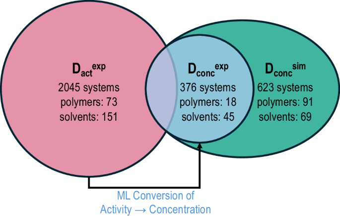
  The pink segment represents the experimental activity-dependent data, labeled as \({D}_{\,\text{act}\,}^{\exp }\), which is converted to a concentration-dependent format using the Sorption Uptake ML model¹⁵. The blue circle denotes the experimental concentration-dependent data, \({D}_{\,\text{conc}\,}^{\exp }\)^{62,63,64,65,66,67,68,69,70,71,72,73,74,75}, while the green segment, \({D}_{\,\text{conc}\,}^{{\rm{sim}}}\), includes concentration-dependent simulated data. These datasets collectively form a comprehensive concentration-dependent diffusivity dataset, comprising 3044 systems, 154 polymers, and 176 solvents, which serves as the foundation for developing the production diffusivity model.

• Augmentation of Simulation Data: The simulated diffusivity dataset, recorded as a function of solvent concentration in the membrane, was fused with the converted experimental concentration-dependent dataset using one-hot encoding, thereby enhancing the diversity of the data.

Together, these augmented datasets created a comprehensive, concentration- and temperature-dependent diffusivity dataset, as illustrated in Fig. 2, which was used to train the diffusivity ML model. Additional data analysis is provided in Supplementary Fig. 1.

ML model benchmarks for improved generalizability

To assess the impact of data fusion and physics-guided learning, we trained and compared both single-task and multi-task diffusivity models across various algorithms. The feature space incorporated Polymer Genome-derived polymer-solvent fingerprints^27,77 (described in Section Polymer and solvent fingerprinting), along with key descriptors such as solvent concentration (expressed as the weight fraction on a logarithmic scale) and temperature. Additionally, one-hot encoded selector vectors were used to distinguish between experimental and simulated data when both were present. Single-task models, trained solely on experimental data, were categorized as ST1 and ST2-based on the amount of data available, as shown in Fig. 3. In contrast, multi-task models combined experimental and simulated data through data fusion. By training on multiple correlated tasks, multi-task learning enables the models to recognize correlations between accurate experimental data and diverse simulated data, expanding prediction capabilities across a broader chemical space. We implemented these models using algorithms such as Gaussian Process Regression (GPR), Neural Networks (NN), and Physics-Enforced Neural Networks (PENN). While GPR and NN modes do not incorporate physical laws into training, the Physics-Enforced Neural Networks (PENN) models incorporate fundamental physical laws into the training process, ensuring that the model reproduces known physical behaviors. Two PENN models were developed. The PENN-1 model is based on an empirically observed relationship where the diffusivity of a solvent decreases with increasing molar volume due to its bulky nature^48,49. This empirical law was initially designed in our previous work to make more accurate predictions for the large solvents (molar volume greater than 1000 cm³/mol) found in real-world crude oil applications, which were absent from the more limited literature-based training dataset that was predominantly distributed around 250 cm³/mol¹⁵. On the other hand, the Arrhenius equation is used to describe the temperature dependence of diffusivity in the PENN-2 model. By embedding the Arrhenius relationship^78,79 within the neural network, we propose improving its predictive accuracy, especially at temperatures outside the range of the training data.

More details about the model architecture are listed in Section Solvent diffusivity ML models.

The model’s performance is evaluated using the Order of Magnitude Error (OME), which is essentially the Mean Absolute Error (MAE) computed on a logarithmic scale^15,29,44. OME is expressed as :

where y_i and \({\hat{y}}_{i}\) represent the actual and predicted values, respectively, and n is the number of data points. The test OME is calculated across various training set sizes using polymer-group splits. These polymer-based “group” splits ensure that test polymers are entirely excluded from training. To ensure statistical reliability, data was split into test-train sets using five different random seeds, with performance statistics reported in Fig. 4, comparing single-task models (ST1 and ST2) and multi-task models trained using GPR, NN, PENN architectures. As expected, test errors decreased as training size increased, eventually plateauing as the models approached their optimal performance.

First, we evaluate the performance of the models as a function of the training data by comparing the performance of single-task (ST1, ST2) and multi-task (MT) models. The ST1 model, trained on the smallest experimental dataset of 2045 polymer-solvent systems, showed the highest test error as a function of training set size (depicted in red in Fig. 4). The ST1 model serves as a baseline to assess the performance of more advanced models. The ST2 model, trained on 2421 experimental systems, was expected to show only modest performance improvements. As shown in green, ST2 models performed similarly to ST1, with slight gains in data-scarce scenarios (10% and 30% trainset sizes). More significant improvements were seen at trainset sizes of 50% and 70%, though the error plateaued at 70%, suggesting that the model was nearing optimal performance, with diminishing returns from additional data. In contrast, the multi-task diffusivity models (shown in blue), trained on a comprehensive dataset of 3,044 systems (combining both experimental and simulated data), significantly outperformed the single-task models. This was especially evident in data-scarce scenarios with as little as 10% trainset data. The multi-task model’s enhanced generalization capabilities stem from leveraging diverse data and learning relationships between experimental and simulated data, underscoring the effectiveness of multi-task learning in improving predictive accuracy in data-limited environments.

Next, we analyzed the effect of different machine-learning algorithms on model performance. In the multi-task (MT) framework, within the data-scarce regime of 10% trainset size, Gaussian Process Regression (GPR) achieved the lowest averaged OME error (0.68), followed by PENN-2 (0.815), with PENN-1 (1.15) and the neural network (NN) model (1.12) showing comparable performance. This indicates that GPR models excel when training data is limited. Furthermore, we note that the limited performance of the PENN2 models in the low-data regime may be attributed to the insufficient coverage of the temperature range in the dataset, which constrains the model’s ability to generalize effectively. Additionally, the complexity of the neural network architecture may contribute to this issue, as more sophisticated models typically require larger datasets to achieve robust generalization. This observation is consistent with previous studies, which have frequently linked performance limitations in such settings to overfitting^80,81,82. However, as more data became available, particularly at 90% trainset size, neural networks significantly outperformed GPR, with errors of 0.179 for NN, 0.173 for PENN-1, 0.164 for PENN-2, and 0.27 for GPR. Notably, as trainset size increased, PENN-2 consistently outperformed other models, especially evident at 50% trainset size. While NN and PENN-1 performed competitively, PENN-2 demonstrated superior predictive power. As discussed in Section Solvent diffusivity ML models, the empirical solvent volume law (equation (4)) incorporated in PENN-1 is particularly effective for large molar volume solvents. However, due to the absence of these larger solvent molecules in the current test dataset (as direct diffusivity measurements were unavailable), the impact of this empirical law was diminished. Consequently, even with the inclusion of physics-based laws, PENN-1 did not reach the performance level of PENN-2. In summary, in data-scarce conditions, the model performance rankings were GPR > PENN-2 > PENN-1 ~ NN. As the training set size increased, this ranking shifted to PENN-2 > PENN-1 ~ NN > GPR. The trends observed in the MT model were similarly reflected in both the ST1 and ST2 models, exhibiting only minor deviations attributable to variability in the train-test splits.

Ultimately, this analysis illustrated that integrating multi-task models with physics-based approaches results in more accurate, robust, and generalizable models, even in scenarios with limited data. Consequently, our production-level diffusivity model was designed as a multi-task model built on a physics-enforced neural network architecture with Arrhenius temperature-dependence encoded (MT-PENN-2).

Comparative production level benchmark

In our previous work¹⁵, we developed a physics-enforced single-task ML model (ST1-PENN-1), using the experimental dataset \({D}_{\,\text{act}\,}^{\exp }\), which covers 2045 polymer-solvent systems. This model predicts polymer-solvent diffusivity based on polymer-solvent fingerprints and solvent activity. In our current work, we expanded this dataset by incorporating additional experimental and simulated data, resulting in a larger dataset of 3044 systems and trained multi-task models using physics-enforced methods (MT-PENN-2). The goal of this updated diffusivity model was to improve generalizability and robustness, enabling accurate predictions in polymer spaces previously unexplored by experiments. In this analysis, we compare the original model (ST1-PENN-1) with the updated model (MT-PENN-2).

Enhanced accuracy from multi-task and physics-enforced learning approaches

As shown in Fig. 4, MT-PENN-2 outperformed ST1-PENN-1, demonstrating superior prediction accuracy across a broader range of polymer chemistries. This success can be attributed to the expanded chemical space from a more diverse dataset (discussed in the following section) and the improved model architecture. It is important to note that ST1-PENN-1 was specifically designed using the PENN-1 architecture to predict diffusivity in large crude oil solvents. While PENN-1 is optimal for such predictions, the PENN-2 architecture excels in predicting solvent diffusivity for smaller organic solvents and new polymer chemistries. However, we note that since the original model of ST-PENN1 used the dataset \({D}_{\,\text{act}}^{\text{exp}\,}\), and this work converted it to a concentration-dependent format \({D}_{\,\text{conc}}^{\text{exp}\,}\), this is not a perfect comparison. This conversion was necessary to ensure consistent units for comparison with other models developed in this study. A direct comparison of models based on activity- or concentration-dependent data could only be made using a test set that overlapped these datasets, which was minimal (only 7 polymers and 84 data points), and this small representation of simple polymers (such as polyethylene) does not accurately reflect the generalizability of the models in the broader chemical space. As a result, we conducted an indirect comparison, and the findings clearly showed that the updated MT-PENN-2 models outperform the original model in prediction accuracy.

Enhanced generalizability due to expanded polymer chemical space

The principal component analysis (PCA) plot using Polymer Genome fingerprints in Fig. 5 demonstrates the broader polymer chemical space covered by the updated diffusivity model (MT-PENN-2) compared to the original model (ST1-PENN-1). The polymer chemical fingerprints are reduced to two dimensions using PCA, capturing the maximum variance and enabling a structured visual representation of the chemical space, wherein each marker represents a unique polymer. The gray markers represent the PCA projection of the fingerprints of a 13k known polymer space. The yellow markers represent the polymer representation for the “original” diffusivity model (ST1-PENN-1) built in our previous work, which was trained solely on experimental data \({D}_{\,\text{act}\,}^{\exp }\)¹⁵. In contrast, the red markers denoting the “updated” diffusivity model (MT-PENN-2) refers to the polymers in the more comprehensive dataset, incorporating \({D}_{\,\text{act}\,}^{\exp }+\,{D}_{\,\text{conc}\,}^{\exp }+\,{D}_{\,\text{conc}\,}^{{\rm{sim}}}\), thus explaining the overlap and expansion in the chemical space.

Overcoming limitations in temperature-dependent-diffusivity predictions

The updated diffusivity model (MT-PENN-2) overcomes a key limitation of the original model by capturing temperature dependence. While the original model was limited to predicting diffusivity near room temperature, the updated model incorporates an Arrhenius-based temperature law, enabling it to extrapolate diffusivity behavior even when temperature-dependent diffusivity data is sparse. This is especially important since most available experimental data is concentrated around room temperature, while many separation applications occur at elevated temperatures. Further details on this improvement have been visualized in Supplementary Fig. 6.

Design guidance for high-performance sustainable membranes

We now aim to identify the ideal pervaporation polymer membrane for separating toluene and heptane by maximizing permeability and ideal permselectivity. This separation is crucial for producing clean motor fuels. The selection of this solvent separation was additionally driven by the availability of extensive training data for this combination to ensure robust and reliable predictions. Toluene-heptane separation is particularly challenging because their physical differences, such as kinetic radius (toluene: 5.9 Å; heptane: 4.42 Å) and boiling point (toluene: 110.6 °C; heptane: 98.4 °C)—are relatively small^83,84. As a result, membrane separations typically depend on exploiting differences in chemical structure and interactions, notably the aromatic nature of toluene versus the aliphatic character of heptane. To address this challenge and guide membrane design, we calculated single-component permeability as the product of ML-predicted diffusivity and solubility coefficients, along with ideal permselectivity as explained in Section Construction of ML based solvent-trade-off plots. This work presents the largest solvent trade-off plots to date, encompassing 13,000 known polymers, along with virtually generated 1 million publicly available polymers in the P1IM database⁵⁷ and 7 million chemically recyclable ring-opening polymerization (ROP) based candidates⁵⁸. Details for this virtual polymer search space can be found in Section Membrane Design Search Space.

Rediscovery of known high-performance candidates

Focusing first on the known polymer space as shown in Fig. 6a (red data points), we present permeability-based trade-off plots, where halogenated polymers (like polyvinyl chloride PVC, denoted by A) emerged as top candidates, exhibiting both high predicted permeability and ideal permselectivity. The diffusivity-based trade-off plot in Fig. 6b, showed similar trends. Figure 6c focuses on solubility, where nitrogen-containing bulky aromatic compounds displayed high solubility and selectivity, likely due to their strong affinity for toluene.

Validating ML-generated trade-off plots is challenging due to limited benchmarking methods. PVC membranes and their composites are recognized for toluene-heptane separations via pervaporation^53,54,55,56. In agreement with literature, our ML predictions independently identified PVC as a top-performing polymer, with a predicted toluene permeability of 10^3.56 Barrer and ideal permselectivity of 10^7.7. The low prediction uncertainties in ML-predicted diffusivity (10^{−9 ± 0.41} cm²/s) and sorption uptake (10^{0.74 ± 0.07} mmol solvent/g polymer) further reinforce the model’s confidence in its predictions, effectively ruling out potential statistical outliers. While the identification of PVC for toluene-heptane separation is not a novel discovery as PVC is well-established in the literature for this separation process, its re-discovery through our ML approach reinforces the validity of our methodology. Further validity is provided by Aouinti et al. who reports PVC’s solubility parameter as 19.2 MPa^1/2, closely matching toluene’s 18.2 MPa^1/2 and significantly differing from heptane’s 15.1 MPa^1/2, implying PVC’s higher affinity for aromatic toluene⁵⁴.

Searching the space of 13k known polymers for non-halogenated alternatives

Despite PVC’s effective separation performance, it is considered one of the most environmentally harmful plastics; thus, identifying sustainable, non-halogenated alternatives is imperative^85,86. To address this, we conducted a systematic screening of 13,000 known polymers to identify non-halogenated candidates with separation performance comparable to PVC. The initial screening was based on a moderately stringent criteria: ideal perm selectivity >10^5.5 and permeability >10⁴ Barrer. To identify non-halogenated alternatives to PVC, we lowered the ideal permselectivity threshold and slightly increased the permeability threshold, as most non-halogenated candidates seemed to show lower ideal permselectivity. However, even the use of this moderately stringent criteria yielded no viable candidates from a dataset of 13k known polymers, underscoring the complexity of the problem-akin to finding a needle in a haystack. In response, we defined a relaxed criteria, such that ideal permselectivity >10⁴ while maintaining the permeability threshold. This shift uncovered 46 candidates, out of which 31 are non-halogenated promising polymers that can be used for toluene-heptane separation. From this pool of polymers, we highlight Polymer B, which emerged as a sustainable candidate, being a known non-halogenated ring-opening polymer with a strong tendency for depolymerization. The rest of the non-halogenated alternative polymers (Supplementary Fig. 7) contain highly polar ester, carbonyl, ketone groups, aromatic or electronegative groups. These trends align with literature findings^53,54,83, as emphasized by Liu et al.⁸⁴, who reviewed 100 membranes for toluene-heptane separation and highlighted that those featuring electronegative groups and aromatic backbones-enabling π–π interactions-exhibit enhanced toluene affinity and separation performance.

Searching the space of chemically recyclable hypothetical polymers

In addition to exploring the known polymer search space to discover sustainable and efficient membranes, we extended our investigation to virtually generated datasets. To ensure reliable predictions, we excluded virtual polymers containing inorganic elements, such as Na, P, and Si, that were absent in the training data.

First, we analyzed the PI1M dataset, comprising 1 million hypothetical polymers, to identify PVC alternatives by applying the moderately stringent screening criteria (ideal permselectivity > 10^5.5, permeability > 10⁴ Barrer). This screening yielded 152 viable polymers, including 74 non-halogenated candidates. As expected, we observe a significant increase in the number of viable candidates with the expansion of chemical space, outlining the importance of such generative design approaches for polymer design. Notably, Polymer C exhibited excellent separation performance, comparable to PVC, with slightly higher permeability, as shown in Fig. 6a. Furthermore, Polymer D emerged as a promising sustainable, non-halogenated alternative. Additionally, applying the relaxed criteria yielded 1243 candidates, of which 920 were non-halogenated. Although a large number of non-halogenated polymers were identified, the chemical space of these polymers closely resembles that of the polymers in PolyInfo⁸⁷, and such polymers may not necessarily be optimized for recycling or represent more sustainable options.

Therefore, recognizing the need for more sustainable membranes, we further explored a dataset of 7 million synthetically accessible ring-opening polymerization (ROP) based polymers with an affinity for chemical recycling. Using the same moderately stringent criteria, we identified 9 candidate polymers, one of which was non-halogenated, denoted as polymer F. We also highlight Polymer E, which is predicted to exhibit slightly better separation performance than PVC. Although Polymer E is halogenated, it demonstrates a strong potential for depolymerization through ROP. Next, while screening for sustainable non-halogenated candidates within this virtual space, we noted that 2.1 million of the polymers were halogenated, significantly narrowing the search space for sustainable alternatives. By using the relaxed screening criteria, we uncovered an additional 114 candidate polymers, of which 48 were non-halogenated (Supplementary Fig. 7). We note that the lower number of candidates passing the screening criteria in the ROP dataset, compared to the PI1M dataset-despite the ROP dataset being nearly seven times larger-may be attributed to its more limited chemical diversity. In contrast, the PI1M dataset benefits from a broader range of chemistries, providing a more diverse pool of potential candidates. We note that while leveraging a virtual space of 8 million polymers-compared to the known space of 13,000-led to the identification of more polymers meeting the specified criteria, the total number of successful candidates remained relatively small, underscoring the inherent complexity and challenges of polymer design. These results point to the fundamental limitations in achieving an optimal permeability-selectivity trade-off, which is primarily influenced by polymer packing and structural factors⁸⁸.

Further, we highlight a discrepancy arising from the ML-based overestimation of ideal diffusivity selectivity and perm-selectivity for the toluene-heptane system. Experimentally, the pervaporation perm-selectivity for a 50/50 multi-component mixture of toluene-heptane at 56 °C is approximately 10.1, significantly lower than the ML-predicted values (Please refer to the Supplementary Information, section 8 for detailed derivations of the formulas and explanations)⁵⁵. This discrepancy underscores a fundamental limitation of ML predictions that rely on single-component transport behavior, and they fail to account for solvent-solvent interactions present in multi-component systems. Previously, we noted that single-component transport behavior is insufficient for describing multi-component systems¹⁵, likely leading to this discrepancy. Furthermore, to assess the validity of the ML predictions, we compared PVC predictions using the published and validated PENN-1 model¹⁵ alongside our PENN-2 models, finding that the predictions closely align, with values for toluene at 10^−8.33 cm²/s and 10^−8.23 cm²/s, and for extremely low values for heptane at 10^−14.01cm²/s and 10^−14.68cm²/s. Thus after eliminating the possibility of invalid ML predictions as the cause of the observed discrepancy, we conduct a more thorough investigation. Aouinti et al. similarly observed the extremely sluggish transport of pure heptane in a modified PVC membrane in their experimental studies, to the extent that flux values could not be measured⁸⁹. Additionally, they reported a significant swelling degree of 49% for PVC in toluene. Based on this, we hypothesize that toluene, due to its strong affinity for PVC, may alter the polymer’s structure by inducing swelling and plasticization, thus creating a more conducive pathway for heptane diffusion. This hypothesis is supported by prior studies; for example, Mathias et al. attributed the loss in diffusivity selectivity to membrane plasticization and introduced the concept of “cohort diffusion”⁹⁰. Here, friction-induced diffusion coupling effects cause faster molecules to slow down and slower molecules to speed up, leading to a reduction in diffusion selectivity. Additionally, Lee et al. observed a loss in diffusivity selectivity when the solubility difference between the polymer and solvents drops below a critical threshold (e.g., δ = 8 MPa^1/2), also attributed to polymer plasticization and swelling⁹¹. These works provide plausible explanations for why the observed selectivities are often much lower than ideal selectivities⁹². In summary, the discrepancy in the ML over-predictions of diffusivity selectivities can be attributed to the absence of solvent-solvent interactions and the effects of polymer swelling. Taking these over-predictions for ideal selectivity into account, we caution against drawing quantitative conclusions from ML predictions for multi-component systems; instead, these models should be used for qualitative insights, such as identifying PVC and other halogenated polymers as strong candidates for this separation.

In addition, we analyzed outlier ML predictions and corresponding prediction uncertainties; incorporating such uncertainty analysis enhances the credibility of ML predictions. By evaluating the standard deviation of predictions across 10 cross-validation (CV) models, we observed higher uncertainty in regions with low permeability and ideal perm-selectivity (Supplementary Fig. 8), indicating that these predictions should be interpreted with caution. Conversely, regions with high permeability and selectivity, which are the primary areas of interest for membrane design, exhibited much lower uncertainties, thus providing greater confidence for exploring new chemical spaces in this regime. In the future, exploring new polymer chemistries and validating the separation performance of these newly discovered polymers through multi-component transport simulations will lay the foundation for developing high-performance, sustainable polymers for solvent separation.